     y    x1 x2  Sex o
1 65.6 174.0  1 Male 1
2 71.8 175.3  1 Male 0
3 80.7 193.5  1 Male 0
4 72.6 186.5  1 Male 0
5 78.8 187.2  1 Male 0
6 74.8 181.5 1 Male 0Missing Data
Prof. Sam Berchuck
Mar 31, 2026
Missing data in research
In any real-world dataset, missing values are nearly always going to be present.
- Missing data can be totally innocuous or a source of bias.
Cannot determine which because there are no values to inspect.
Handling missing data is extremely difficult!
Example
Suppose an individual’s depression scores are missing in dataset of patients with colon cancer.
It could be missing because:
A data entry error where some values did not make it into the dataset.
The patient is a man, and men are less likely to complete the depression score in general (i.e., it is not related to the unobserved depression).
The patient has depression and as a result did not complete the depression survey.
Classifactions of missing data
Missing completely at random (MCAR)
- This is the ideal case but rarely seen in practice. Usually a data entry problem.
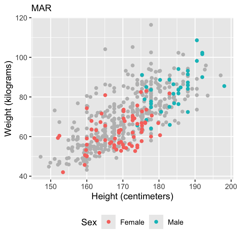
Missing at random (MAR)
- The missing value is related to some other variable that has been collected.
Missing not at random (MNAR)
- The missing value is related to a variable that was not collected or not observed.
Missing data
Missing data can appear in the outcome and/or predictors.
Today, we will write down some math for missing data occuring in the outcome space, however this is generalizable to missingness in the predictor space.
Missing data framework
We are interested in modeling a random variable \(Y_{i}\), for \(i \in \{1,\ldots,n\}\).
In a missing data setting, we only observe the outcome in a subset of observations, \(\mathbf{Y}_{obs} = \{Y_{i}:i \in \mathcal N_{obs}\}\).
- \(\mathcal N_{obs}\) is the set of indeces in the observed set, such that \(|\mathcal N_{obs}|= n_{obs}\) is the number of observed data points.
The remaining observations are assumed to be missing and are contained in \(\mathbf{Y}_{mis} = \{Y_{i}:i \in \mathcal N_{mis}\}\).
- \(\mathcal N_{mis}\) is the set of indeces of the missing data and \(|\mathcal N_{mis}|= n_{mis}\) is the number of missing data points.
The full set of data is given by \(\mathbf{Y}=(\mathbf{Y}_{obs},\mathbf{Y}_{mis})\).
Missing data notation
Define \(O_{i}\) as a binary indicator of observation \(Y_{i}\) being present, where \(O_{i} = 1\) indicates that \(Y_{i}\) was observed.
The collection of missingness indicators is given by \(\mathbf{O} = \{O_{i}:i = 1,\ldots,n\}\).
Our observed data then consists of \((\mathbf{Y}_{obs}, \mathbf{O})\).
Complete data likelihood
- The joint distribution of \((\mathbf{Y}, \mathbf{O})\) can be written as,
\[f(\mathbf{Y}, \mathbf{O} | \mathbf{X}, \boldsymbol{\theta},\boldsymbol{\phi}) = \underbrace{f(\mathbf{Y} | \mathbf{X}, \boldsymbol{\theta})}_{\text{likelihood}} \times \underbrace{f(\mathbf{O} | \mathbf{Y}, \mathbf{X}, \boldsymbol{\phi})}_{\text{missing model}}.\]
The parameter block, \((\boldsymbol{\theta},\boldsymbol{\phi})\), consists of:
\(\boldsymbol{\theta}\), the target parameters of interest (e.g., feature effects on outcome), and
\(\boldsymbol{\phi}\), the nuisance parameters.
Can we perform inference using this likelihood?
Observed data likelihood
- The likelihood for the observed data must be written by marginalizing over the unobserved outcome variables.
\[\begin{aligned} f(\mathbf{Y}_{obs}, \mathbf{O} | \mathbf{X}, \boldsymbol{\theta},\boldsymbol{\phi}) &= \int f(\mathbf{Y}_{obs}, \mathbf{Y}_{mis}, \mathbf{O} | \mathbf{X}, \boldsymbol{\theta},\boldsymbol{\phi}) d\mathbf{Y}_{mis}\\ &= \int f(\mathbf{Y}, \mathbf{O} |\mathbf{X}, \boldsymbol{\theta},\boldsymbol{\phi}) d\mathbf{Y}_{mis}\\ &= \int \underbrace{f(\mathbf{Y} |\mathbf{X}, \boldsymbol{\theta}) f(\mathbf{O} | \mathbf{X},\mathbf{Y}, \boldsymbol{\phi})}_{\text{complete data likelihood}} d\mathbf{Y}_{mis} \end{aligned}\]
Missing data models: MCAR
The data are missing completely at random (MCAR) if the missing mechanism is defined as, \[\begin{aligned} f(\mathbf{O} | \mathbf{Y},\mathbf{X},\boldsymbol{\phi}) &= f(\mathbf{O} | \mathbf{Y}_{obs}, \mathbf{Y}_{mis},\mathbf{X},\boldsymbol{\phi})\\ &= f(\mathbf{O} | \boldsymbol{\phi}). \end{aligned}\]
- The missingness does not depend on any data.
Implications of the missing model: MCAR
\[\begin{aligned} f(\mathbf{Y}_{obs}, \mathbf{O} |\mathbf{X}, \boldsymbol{\theta},\boldsymbol{\phi}) &= \int f(\mathbf{Y} | \mathbf{X},\boldsymbol{\theta}) f(\mathbf{O} | \mathbf{Y}, \mathbf{X},\boldsymbol{\phi}) d\mathbf{Y}_{mis}\\ &= \int f(\mathbf{Y} | \mathbf{X},\boldsymbol{\theta}) f(\mathbf{O} | \boldsymbol{\phi}) d\mathbf{Y}_{mis}\\ &= f(\mathbf{O} | \boldsymbol{\phi}) \int f(\mathbf{Y}_{obs} |\mathbf{X}_{obs}, \boldsymbol{\theta}) f(\mathbf{Y}_{mis} |\mathbf{X}_{mis}, \boldsymbol{\theta})d\mathbf{Y}_{mis}\\ &= f(\mathbf{Y}_{obs} | \mathbf{X}_{obs},\boldsymbol{\theta})f(\mathbf{O} | \boldsymbol{\phi})\int f(\mathbf{Y}_{mis} |\mathbf{X}_{mis}, \boldsymbol{\theta}) d\mathbf{Y}_{mis}\\ &= f(\mathbf{Y}_{obs} | \mathbf{X}_{obs},\boldsymbol{\theta})f(\mathbf{O} | \boldsymbol{\phi}). \end{aligned}\]
Key points about MCAR assumption
No bias: The analysis based on the observed data will not be biased, as the missingness does not systematically favor any particular pattern in the data.
Reduced power: While unbiased, MCAR still reduces the statistical power of the analysis due to the smaller sample size resulting from missing data.
Simple handling methods: Because of its random nature, MCAR allows for straightforward handling methods like listwise deletion (i.e., complete-case analysis) or simple imputation techniques (e.g., mean imputation) without introducing bias.
Missing data models: MAR
The data are missing at random (MAR) if the missing mechanism is defined as, \[\begin{aligned} f(\mathbf{O} | \mathbf{Y},\mathbf{X},\boldsymbol{\phi}) &= f(\mathbf{O} | \mathbf{Y}_{obs}, \mathbf{Y}_{mis},\mathbf{X},\boldsymbol{\phi})\\ &= f(\mathbf{O} | \mathbf{Y}_{obs},\mathbf{X},\boldsymbol{\phi}). \end{aligned}\]
- The missingness depends on the observed data only.
Implications of the missing model: MAR
\[\begin{aligned} f(\mathbf{Y}_{obs}, \mathbf{O} |\mathbf{X}, \boldsymbol{\theta},\boldsymbol{\phi}) &= \int f(\mathbf{Y} |\mathbf{X}, \boldsymbol{\theta}) f(\mathbf{O} | \mathbf{Y},\mathbf{X}, \boldsymbol{\phi}) d\mathbf{Y}_{mis}\\ &\hspace{-2in}= \int f(\mathbf{Y} | \mathbf{X},\boldsymbol{\theta}) f(\mathbf{O} | \mathbf{Y}_{obs},\mathbf{X}, \boldsymbol{\phi}) d\mathbf{Y}_{mis}\\ &\hspace{-2in}= f(\mathbf{O} | \mathbf{Y}_{obs},\mathbf{X},\boldsymbol{\phi}) \int f(\mathbf{Y}_{obs} | \mathbf{X}_{obs},\boldsymbol{\theta}) f(\mathbf{Y}_{mis} | \mathbf{X}_{mis},\boldsymbol{\theta})d\mathbf{Y}_{mis}\\ &\hspace{-2in}= f(\mathbf{Y}_{obs} |\mathbf{X}_{obs}, \boldsymbol{\theta})f(\mathbf{O} |\mathbf{Y}_{obs},\mathbf{X}, \boldsymbol{\phi})\int f(\mathbf{Y}_{mis} | \mathbf{X}_{mis},\boldsymbol{\theta}) d\mathbf{Y}_{mis}\\ &\hspace{-2in}= f(\mathbf{Y}_{obs} | \mathbf{X}_{obs},\boldsymbol{\theta})f(\mathbf{O} |\mathbf{Y}_{obs}, \mathbf{X},\boldsymbol{\phi}). \end{aligned}\]
- Unbiased Parameter Estimates: Similar to MCAR, we can perform a complete case analysis and can ignore the missing data model! This is never done, however, because it leads to incorrect inference.
Key points about MAR assumption
Complete-case analysis is not acceptable:
Parameter estimation remains unbiased, but, in general, estimation of variances and intervals is biased.
Also, smaller sample size leads to less power and worse prediction.
Under certain missingness settings, parameter estimation may not be unbiased.
Simple handling approaches fail: Methods like mean imputation will also result in small estimated standard errors.
More advanced methods are needed: Multiple imputation, Bayes.
Missing data models: MNAR
The data are missing not at random (MNAR) if the missing mechanism is defined as, \[\begin{aligned} f(\mathbf{O} | \mathbf{Y},\mathbf{X},\boldsymbol{\phi}) &= f(\mathbf{O} | \mathbf{Y}_{obs}, \mathbf{Y}_{mis},\mathbf{X},\boldsymbol{\phi}). \end{aligned}\]
- The missingness depends on the observed and missing data.
Implications of the missing model: MNAR
\[\begin{aligned} f(\mathbf{Y}_{obs}, \mathbf{O} | \mathbf{X},\boldsymbol{\theta},\boldsymbol{\phi}) &= \int f(\mathbf{Y} | \mathbf{X},\boldsymbol{\theta}) f(\mathbf{O} | \mathbf{Y},\mathbf{X}, \boldsymbol{\phi}) d\mathbf{Y}_{mis}\\ &\hspace{-2in}= \int f(\mathbf{Y} | \mathbf{X},\boldsymbol{\theta}) f(\mathbf{O} | \mathbf{Y}_{obs},\mathbf{Y}_{mis}, \mathbf{X},\boldsymbol{\phi}) d\mathbf{Y}_{mis}\\ &\hspace{-2in}= \int f(\mathbf{Y}_{obs} |\mathbf{X}_{obs}, \boldsymbol{\theta}) f(\mathbf{Y}_{mis} | \mathbf{X}_{mis},\boldsymbol{\theta})f(\mathbf{O} | \mathbf{Y},\mathbf{X},\boldsymbol{\phi})d\mathbf{Y}_{mis}\\ &\hspace{-2in}= f(\mathbf{Y}_{obs} | \mathbf{X}_{obs},\boldsymbol{\theta}) \int f(\mathbf{Y}_{mis} | \mathbf{X}_{mis},\boldsymbol{\theta})f(\mathbf{O} | \mathbf{Y},\mathbf{X},\boldsymbol{\phi})d\mathbf{Y}_{mis} \end{aligned}\]
Under the MNAR assumption, we are NOT allowed to ignore the missing data. We must specify a model for the missing data.
This is really hard! We can ignore this in our class.
Summary of missing mechanisms
Under MCAR and MAR, we are allowed to fit our model to the observed data (i.e., a complete case analysis/listwise deletion). Under these settings the missingness is considered ignorable.
Under MAR, fitting the complete case analysis is not efficient and advanced techniques are needed to guarentee proper statistical inference.
Under MNAR, we must model the missing data mechanism. This data is considered non-ignorable.
Bayesian approches to missing data
- Full Bayesian joint model
- Multiple imputation
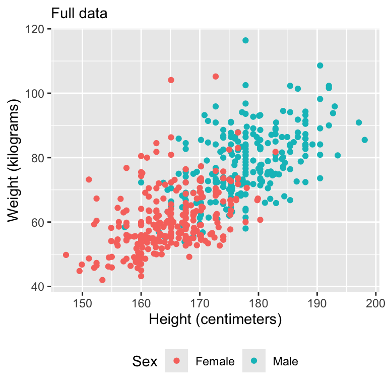
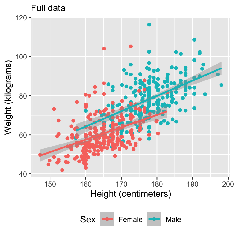
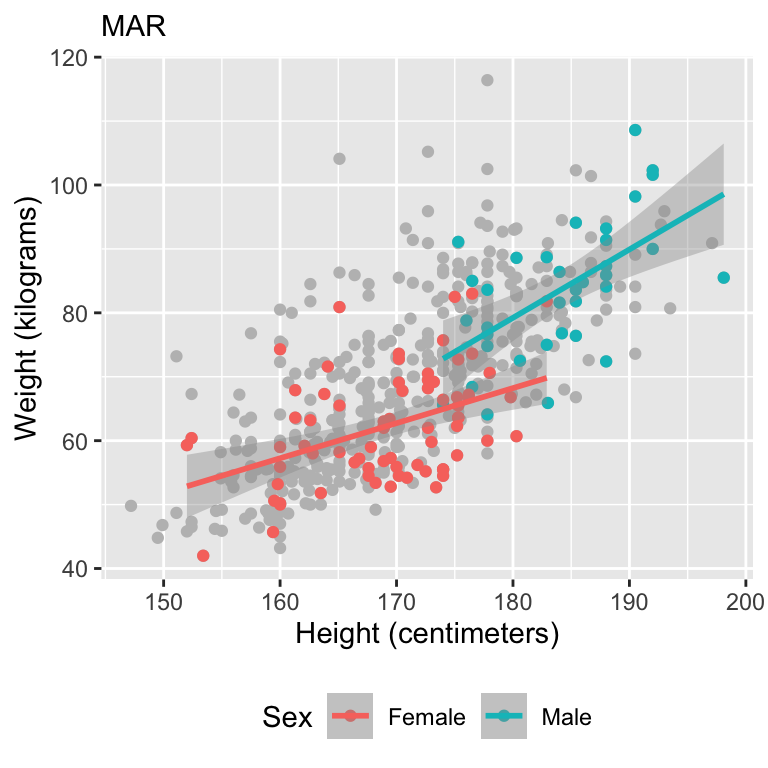
Let’s motivate with some data
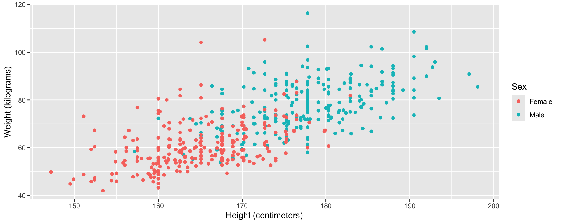
Simulate missing data
Visualize data
Model fits
Full Bayesian model
- Since we are Bayesians, we can treat the unobserved \(\mathbf{Y}_{mis}\) as parameters and work with the complete data likelihood.
\[\begin{aligned} f(\boldsymbol{\theta}, \boldsymbol{\phi}, \mathbf{Y}_{mis} | \mathbf{Y}_{obs},\mathbf{O},\mathbf{X}) &\propto f(\mathbf{Y}, \mathbf{O}, \boldsymbol{\theta}, \boldsymbol{\phi} | \mathbf{X})\\ &\hspace{-4in}=f(\mathbf{Y}, \mathbf{O} | \mathbf{X}, \boldsymbol{\theta},\boldsymbol{\phi})f(\boldsymbol{\theta},\boldsymbol{\phi})\\ &\hspace{-4in}= f(\mathbf{Y} | \mathbf{X}, \boldsymbol{\theta})f(\mathbf{O} | \mathbf{Y}, \mathbf{X}, \boldsymbol{\phi})f(\boldsymbol{\theta},\boldsymbol{\phi})\\ &\hspace{-4in}=f(\mathbf{Y}_{obs} | \mathbf{X}_{obs}, \boldsymbol{\theta})f(\mathbf{Y}_{mis} | \mathbf{X}_{mis}, \boldsymbol{\theta})f(\mathbf{O} | \mathbf{Y}, \mathbf{X}, \boldsymbol{\phi})f(\boldsymbol{\theta},\boldsymbol{\phi})\\ \end{aligned}\]
- We can simplify this posterior by dropping the missing data mechanism.
Full Bayesian model
- Assuming that \(f(\boldsymbol{\theta},\boldsymbol{\phi}) = f(\boldsymbol{\theta})f(\boldsymbol{\phi})\), the missingness process does not need to be explicitly modeled when we are interested in inference for \(\boldsymbol{\theta}\).
\[\begin{aligned} &f(\boldsymbol{\theta}, \mathbf{Y}_{mis} | \mathbf{Y}_{obs},\mathbf{O},\mathbf{X})\\ &\hspace{2in}\propto f(\mathbf{Y}_{obs} | \mathbf{X}_{obs}, \boldsymbol{\theta})f(\mathbf{Y}_{mis} | \mathbf{X}_{mis}, \boldsymbol{\theta})f(\boldsymbol{\theta}) \end{aligned}\]
Full Bayesian model for linear regression
\[\begin{aligned} Y_i | \alpha, \beta, \sigma^2 &\stackrel{ind}{\sim} N(\alpha + \mathbf{x}_i\boldsymbol{\beta}, \sigma^2), \quad i \in \mathcal N_{obs}\\ Y_i | \alpha, \beta, \sigma^2&\stackrel{ind}{\sim} N(\alpha + \mathbf{x}_i \boldsymbol{\beta}, \sigma^2), \quad i \in \mathcal N_{mis}\\ \alpha &\sim f(\alpha)\\ \beta &\sim f(\boldsymbol{\beta})\\ \sigma &\sim f(\sigma), \end{aligned}\]
- \(\mathbf{x}_i = (height_i, 1(sex_i = male), height_i \times 1(sex_i = male))\).
Full Bayesian missing data model in Stan
// saved in missing-full-bayes.stan
data {
  int<lower = 1> n_obs;
  int<lower = 1> n_mis;
  int<lower = 1> p;
  vector[n_obs] Y_obs;
  matrix[n_obs, p] X_obs;
  matrix[n_mis, p] X_mis;
}
transformed data {
  vector[n_obs] Y_obs_centered;
  real Y_bar;
  matrix[n_obs, p] X_obs_centered;
  matrix[n_mis, p] X_mis_centered;
  row_vector[p] X_bar;
  Y_bar = mean(Y_obs);
  Y_obs_centered = Y_obs - Y_bar;
  matrix[n_obs + n_mis, p] X = append_row(X_obs, X_mis);
  for (i in 1:p) {
    X_bar[i] = mean(X[, i]);
    X_obs_centered[, i] = X_obs[, i] - X_bar[i];
    X_mis_centered[, i] = X_mis[, i] - X_bar[i];
  }
}
parameters {
  real alpha_centered;
  vector[p] beta;
  real<lower = 0> sigma;
  vector[n_mis] Y_mis_centered;
}
model {
  target += normal_lpdf(Y_obs_centered | alpha_centered + X_obs_centered * beta, sigma);
  target += normal_lpdf(Y_mis_centered | alpha_centered + X_mis_centered * beta, sigma);
  target += normal_lpdf(alpha_centered | 0, 10);
  target += normal_lpdf(beta | 0, 10);
  sigma ~ normal(0, 10);
}
generated quantities {
  real alpha;
  vector[n_mis] Y_mis;
  alpha = Y_bar + alpha_centered - X_bar * beta;
  Y_mis = Y_mis_centered + Y_bar;
}
Fit missing data model
stan_missing_data_model <- stan_model(file = "missing-full-bayes.stan")
X <- model.matrix(~ x1 * x2, data = fulldata)[, -1]
stan_data_missing_data <- list(
  n_obs = sum(fulldata$o == 1),
  n_mis = sum(fulldata$o == 0),
  p = ncol(X),
  Y_obs = array(fulldata$y[fulldata$o == 1]),
  X_obs = X[fulldata$o == 1, ],
  X_mis = X[fulldata$o == 0, ]
)
fit_full_bayes_joint <- sampling(stan_missing_data_model, stan_data_missing_data)
Explore model fit
Inference for Stan model: anon_model.
4 chains, each with iter=2000; warmup=1000; thin=1;
post-warmup draws per chain=1000, total post-warmup draws=4000.
mean se_mean sd 2.5% 97.5% n_eff Rhat
alpha -48.38 0.83 21.10 -90.15 -7.03 653 1.00
beta[1] 0.65 0.00 0.12 0.41 0.90 673 1.00
beta[2] -3.19 0.22 9.75 -22.23 16.56 2047 1.00
beta[3] 0.08 0.00 0.06 -0.03 0.19 2487 1.00
sigma 8.21 0.02 0.58 7.17 9.45 600 1.01
Samples were drawn using NUTS(diag_e) at Wed Jan 22 19:43:45 2025.
For each parameter, n_eff is a crude measure of effective sample size,
and Rhat is the potential scale reduction factor on split chains (at
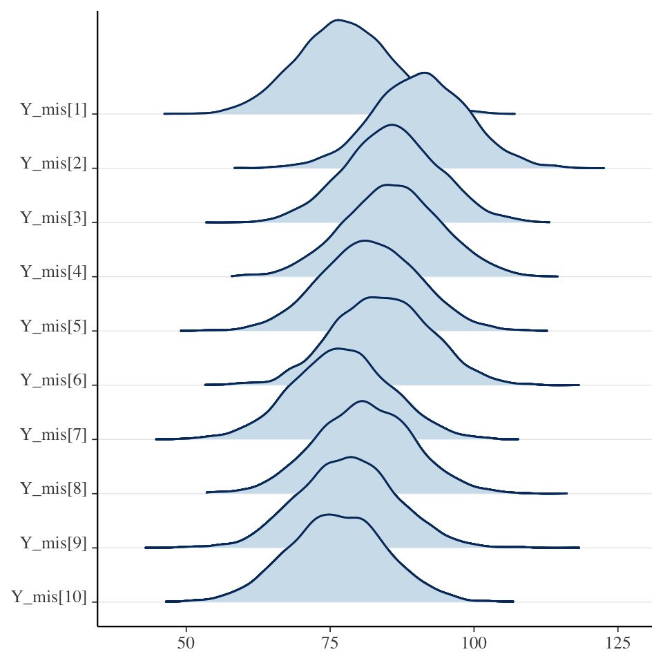
convergence, Rhat=1).Explore latent missing variable
Summary of Bayesian joint model
The joint model treats the missing data as parameters (i.e., latent variables in the model).
Placing a prior on the missing data allows us to jointly learn the model parameters and the missing data.
Equivalent to multiple imputation at every step of the HMC. Can be slow!
In Stan, we can only treat continuous missing data as parameters, so this method is somewhat limited (what do we do if the missing data is a binary outcome?)
Multiple imputation
As an alternative to fitting a joint model, there are many approaches that allow us to impute missing data before the actual model fitting takes place.
Each missing value is not imputed once but \(m\) times leading to a total of \(m\) fully imputed data sets.
The model can then be fitted to each of those data sets separately and results are pooled across models, afterwards.
One widely applied package for multiple imputation is
mice(Buuren & Groothuis-Oudshoorn, 2010) and we will use it in combination with Stan.
Mice
- Here, we apply the default settings of mice, which means that all variables will be used to impute missing values in all other variables and imputation functions automatically chosen based on the variables’ characteristics.
Mice
Now, we have \(m = 100\) imputed data sets stored within the
impobject.- In practice, we will likely need more than 5 of those to accurately account for the uncertainty induced by the missingness, perhaps even in the area of 100 imputed data sets (Zhou & Reiter, 2010).
We can extract the first imputed dataset.
- We can now fit our model \(m\) times for each imputed data sets and combine the posterior samples from all chains for inference.
Model for the imputed datasets
// bayesian-mi.stan
data {
  int<lower = 1> n;
  int<lower = 1> p;
  vector[n] Y;
  matrix[n, p] X;
}
transformed data {
  vector[n] Y_centered;
  real Y_bar;
  matrix[n, p] X_centered;
  row_vector[p] X_bar;
  Y_bar = mean(Y);
  Y_centered = Y - Y_bar;
  for (i in 1:p) {
    X_bar[i] = mean(X[, i]);
    X_centered[, i] = X[, i] - X_bar[i];
  }
}
parameters {
  real alpha_centered;
  vector[p] beta;
  real<lower = 0> sigma;
}
model {
  target += normal_lpdf(Y_centered | alpha_centered + X_centered * beta, sigma);
  target += normal_lpdf(alpha_centered | 0, 10);
  target += normal_lpdf(beta | 0, 10);
  sigma ~ normal(0, 10);
}
generated quantities {
  real alpha;
  alpha = Y_bar + alpha_centered - X_bar * beta;
}
Fit the model to the imputed data
stan_bayesian_mi <- stan_model(file = "bayesian-mi.stan")
alpha <- beta <- sigma <- r_hat <- n_eff <- NULL
n_chains <- 2
for (i in 1:m) {
###Load each imputed dataset and fit the Stan complete case model
data <- complete(imp, i)
X <- model.matrix(~ x1 * x2, data = data)[, -1, drop = FALSE]
stan_data_bayesian_mi <- list(
n = nrow(data),
p = ncol(X),
Y = data$y,
X = X
)
fit_mi <- sampling(stan_bayesian_mi, stan_data_bayesian_mi, chains = n_chains)
###Save convergence diagnostics from each imputed dataset
r_hat <- cbind(r_hat, summary(fit_mi)$summary[, "Rhat"])
n_eff <- cbind(n_eff, summary(fit_mi)$summary[, "n_eff"])
pars <- rstan::extract(fit_mi, pars = c("alpha", "beta", "sigma"))
### Save the parameters from each imputed dataset
n_sims_chain <- length(pars$alpha) / n_chains
alpha <- rbind(alpha, cbind(i, rep(1:n_chains, each = n_sims_chain), pars$alpha))
beta <- rbind(beta, cbind(i, rep(1:n_chains, each = n_sims_chain), pars$beta))
sigma <- rbind(sigma, cbind(i, rep(1:n_chains, each = n_sims_chain), pars$sigma))
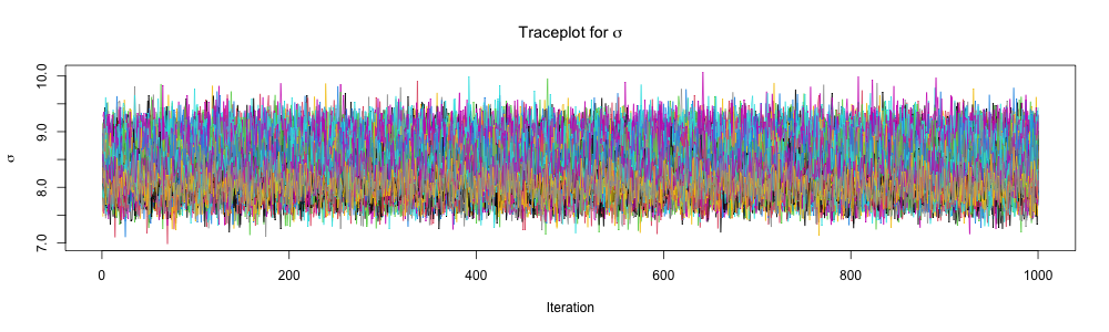
}Inspect traceplots
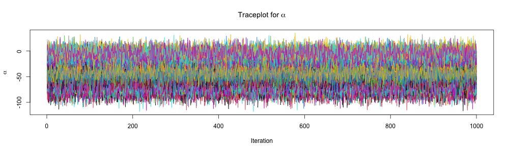
Inspect traceplots
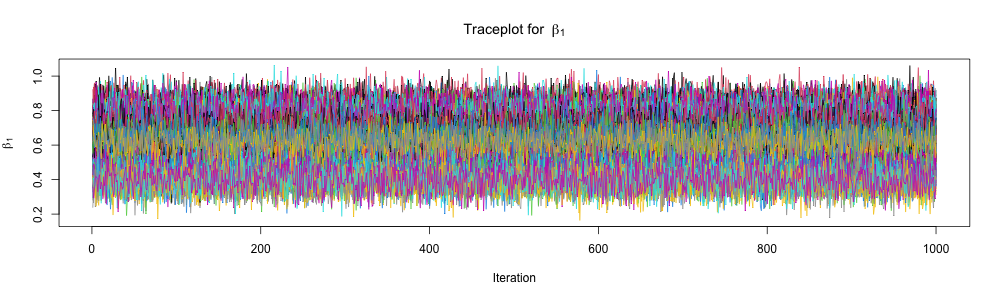
Inspect traceplots
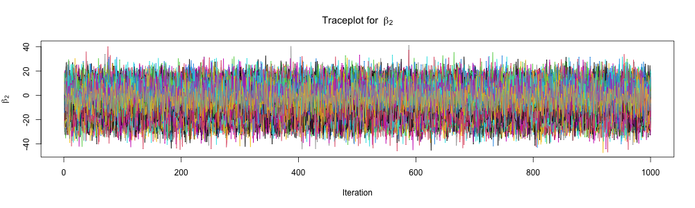
Inspect traceplots
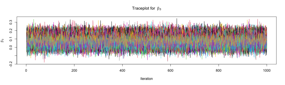
Inspect traceplots
Comparison of methods: \(\alpha\)
| Data | Model | Mean | SD | 2.5% | 97.5% | n_eff | Rhat |
|---|---|---|---|---|---|---|---|
| Full | OLS | -43.82 | 13.78 | -70.89 | -16.75 | NA | NA |
| MAR | Bayes Joint | -48.38 | 21.10 | -90.15 | -7.03 | 652.73 | 1 |
| MAR | Bayes MI | -43.45 | 23.72 | -85.03 | 3.97 | 119974.91 | 1 |
| MAR | OLS | -30.56 | 23.70 | -77.55 | 16.43 | NA | NA |
Comparison of methods: \(\beta_1\)
| Data | Model | Mean | SD | 2.5% | 97.5% | n_eff | Rhat |
|---|---|---|---|---|---|---|---|
| Full | OLS | 0.63 | 0.08 | 0.47 | 0.80 | NA | NA |
| MAR | Bayes Joint | 0.65 | 0.12 | 0.41 | 0.90 | 672.77 | 1 |
| MAR | Bayes MI | 0.63 | 0.14 | 0.35 | 0.87 | 119778.47 | 1 |
| MAR | OLS | 0.55 | 0.14 | 0.27 | 0.83 | NA | NA |
Comparison of methods: \(\beta_2\)
| Data | Model | Mean | SD | 2.5% | 97.5% | n_eff | Rhat |
|---|---|---|---|---|---|---|---|
| Full | OLS | -17.13 | 19.56 | -55.57 | 21.30 | NA | NA |
| MAR | Bayes Joint | -3.19 | 9.75 | -22.23 | 16.56 | 2047.43 | 1 |
| MAR | Bayes MI | -5.52 | 10.24 | -25.29 | 14.89 | 85499.19 | 1 |
| MAR | OLS | -82.60 | 49.54 | -180.82 | 15.62 | NA | NA |
Comparison of methods: \(\beta_3\)
| Data | Model | Mean | SD | 2.5% | 97.5% | n_eff | Rhat |
|---|---|---|---|---|---|---|---|
| Full | OLS | 0.15 | 0.11 | -0.08 | 0.37 | NA | NA |
| MAR | Bayes Joint | 0.08 | 0.06 | -0.03 | 0.19 | 2487.34 | 1 |
| MAR | Bayes MI | 0.09 | 0.06 | -0.03 | 0.20 | 83444.33 | 1 |
| MAR | OLS | 0.52 | 0.27 | -0.02 | 1.06 | NA | NA |
Comparison of methods: \(\sigma\)
| Data | Model | Mean | SD | 2.5% | 97.5% | n_eff | Rhat |
|---|---|---|---|---|---|---|---|
| Full | OLS | 8.73 | 0.39 | 8.07 | 9.49 | NA | NA |
| MAR | Bayes Joint | 8.21 | 0.58 | 7.17 | 9.45 | 599.95 | 1.01 |
| MAR | Bayes MI | 8.36 | 0.35 | 7.71 | 9.09 | 151152.94 | 1.00 |
| MAR | OLS | 7.87 | 0.52 | 6.84 | 8.90 | NA | NA |
Prepare for next class
Work on HW 05.
Complete reading to prepare for Thursday’s lecture
Thursday’s lecture: Bayesian Clustering