u = center(observed and prediction locations)
S = box size (u)
max_iter = 30

# initialization
j = 0
check = FALSE
diagnosis = logical(max_iter) # store checking results for each iteration

# initial guess
rho = 0.5*S # recommended initial value
c = minimum c given rho
m = minimum m given c, and rho
B = c*S

while (!check & j<=max_iter){

  fit = runHSGP(B,m) # stan run
  j = j + 1

  rho_hat = mean(fit$rho) # obtain fitted value for rho
  # check the fitted is larger than the minimum rho that can be well approximated
  diagnosis[j] = (rho_hat + 0.01 >= rho)
  if (j==1) {
    if (diagnosis[j]){
      # if the diagnosis check is passed, do one more run just to make sure
      m = m + 2
      update c using rho_hat
      update rho using m and c
    } else {
      # if the check failed, update our knowledge about rho
      rho = rho_hat
      update c and m using rho_hat
    }
  } else {
    if (diagnosis[j] & diagnosis[j-2]){
      # if the check passed for the last two runs, we finish tuning
      check = TRUE
    } else if (diagnosis[j] & !diagnosis[j-2]){
      # if the check failed last time but passed this time, do one more run
      m = m + 2
      update c using rho_hat
      update rho using m and c
    } else if (!diagnosis[j]){
      # if the check failed, update our knowledge about rho
      rho = rho_hat
      update c and m using rho_hat
    }
  }
  B = c*S
}Scalable Gaussian Processes #2
Christine Shen
Mar 24, 2026
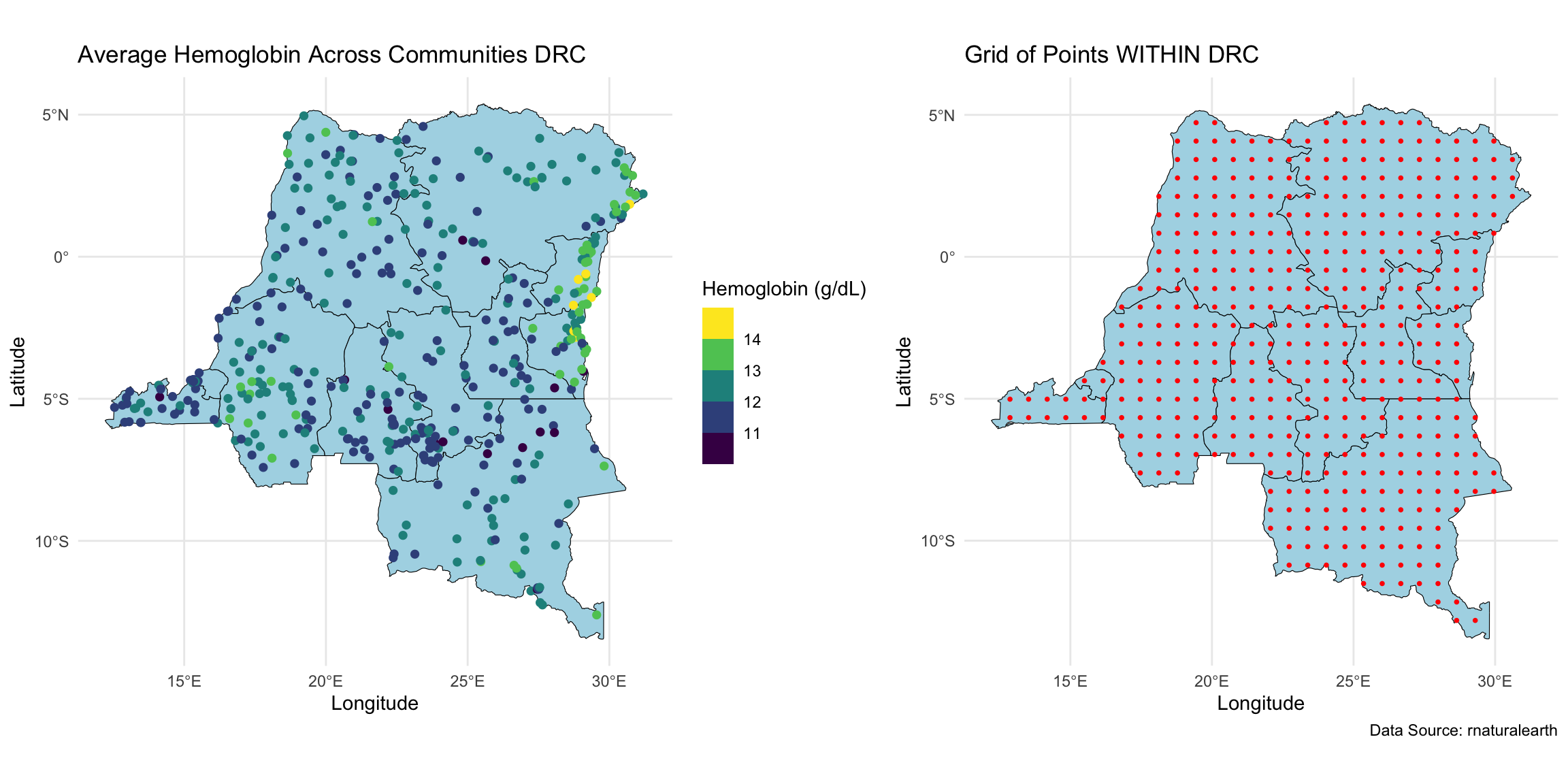
Geospatial analysis on hemoglobin dataset
We wanted to perform geospatial analysis on a dataset with ~8,600 observations at ~500 locations, and make predictions at ~440 locations on a grid.
Geospatial model
We specify the following model: \[\mathbf{Y} = \alpha \mathbf{1}_{N} + \mathbf{X} \boldsymbol{\beta} + \mathbf{Z}\boldsymbol{\theta} + \boldsymbol{\epsilon}, \quad \boldsymbol{\epsilon} \sim N_N(\mathbf{0},\sigma^2\mathbf{I})\] with priors
- \(\boldsymbol{\theta}(\mathbf{u}) | \tau,\rho \sim GP(\mathbf{0},C(\cdot,\cdot))\), where \(C\) is the Matérn 3/2 covariance function with magnitude \(\tau\) and length scale \(\rho\)
- \(\alpha^* \sim N(0,4^2)\). This is the intercept after centering \(\mathbf{X}\).
- \(\beta_j | \sigma_{\beta} \sim N(0,\sigma_{\beta}^2)\), \(j \in \{1,\dots,p\}\)
- \(\sigma \sim \text{Half-Normal}(0, 2^2)\)
- \(\tau \sim \text{Half-Normal}(0, 4^2)\)
- \(\rho \sim \text{Inv-Gamma}(5, 5)\)
- \(\sigma_{\beta} \sim \text{Half-Normal}(0, 2^2)\)
Review of the last lecture
Gaussian process (GP) is not scalable as it requires \(\mathcal{O}(n^3)\) flops per MCMC iteration.
Introduced HSGP, a Hilbert space low-rank approximation method for GP. \[\mathbf{C} \approx \boldsymbol{\Phi}\mathbf{S}\boldsymbol{\Phi}^T, \quad \text{where}\]
- feature matrix \(\boldsymbol{\Phi} \in \mathbb{R}^{n \times m}\) only depends on the approximation box \(B\) and observed locations.
- diagonal matrix \(\mathbf{S} \in \mathbb{R}^{m \times m}\) only depends on the covariance function \(C\) and its parameters \(\tau\) and \(\rho\).
- \(m\) is the number of basis functions.
Model reparameterization under HSGP: \(\boldsymbol{\theta} \overset{d}{=} \boldsymbol{\Phi} \mathbf{S}^{1/2}\mathbf{b}\), \(\mathbf{b} \sim N_m(0,\mathbf{I})\).
How to do posterior sampling under HSGP in
stan
Review of the last lecture
How to do kriging under HSGP in
stanUnder the reparameterized model, \(\boldsymbol{\theta} = \boldsymbol{\Phi} \mathbf{S}^{1/2}\mathbf{b}\), where \(\mathbf{b}\) is treated as the unknown parameter, and \(S\) is known given \(\tau\) and \(\rho\). Therefore for kriging:
\[\begin{align} \boldsymbol{\theta}^* \mid (\boldsymbol{\theta},\boldsymbol{\Omega}) &= \boldsymbol{\Phi}^*\mathbf{S}^{1/2}\mathbf{b} \mid (\mathbf{b},\boldsymbol{\Omega}) \\ &=\boldsymbol{\Phi}^*\mathbf{S}^{1/2}\mathbf{b}. \end{align}\]
During MCMC sampling, we can obtain posterior predictive samples for \(\boldsymbol{\theta}^*\) through posterior samples of \(\mathbf{b}\) and \(\mathbf{S}\). Let superscript \((s)\) denote the \(s\)th posterior sample:
\[\boldsymbol{\theta}^{*(s)} = \boldsymbol{\Phi}^* \mathbf{S}^{(s) 1/2} \mathbf{b}^{(s)}.\]
Kriging under HSGP
Under HSGP: \[\begin{align} \begin{bmatrix} \boldsymbol{\theta} \\ \boldsymbol{\theta}^* \end{bmatrix} \Bigg| \boldsymbol{\Omega} \sim N_{n +q} \left(\begin{bmatrix} \mathbf{0}_n \\ \mathbf{0}_q \end{bmatrix}, \begin{bmatrix} \boldsymbol{\Phi}\mathbf{S}\boldsymbol{\Phi}^\top & \boldsymbol{\Phi}\mathbf{S} \boldsymbol{\Phi}^{*\top} \\ \boldsymbol{\Phi}^*\mathbf{S}\boldsymbol{\Phi}^\top & \boldsymbol{\Phi}^*\mathbf{S}\boldsymbol{\Phi}^{*\top} \end{bmatrix} \right). \end{align}\]
If \(m \le n\), we have shown \[\boldsymbol{\theta}^* \mid (\boldsymbol{\theta}, \boldsymbol{\Omega}) = (\boldsymbol{\Phi}^*\mathbf{S}\boldsymbol{\Phi}^\top) (\boldsymbol{\Phi}\mathbf{S}\boldsymbol{\Phi}^\top)^{\dagger} \boldsymbol{\theta}\overset{d}{=}\boldsymbol{\Phi}^*\mathbf{S}^{1/2}\mathbf{b}.\]
Now we show if \(m>n\), \(\boldsymbol{\theta}^* \mid (\boldsymbol{\theta}, \boldsymbol{\Omega}) \overset{d}{=}\boldsymbol{\Phi}^*\mathbf{S}^{1/2}\mathbf{b}.\)
HSGP parameters
How to choose
- number of basis functions \(m\)
- the approximation box \(B\)
Solin and Särkkä (2020) showed that HSGP approximation can be made arbitrarily accurate as \(B\) and \(m\) increase.
Our goal:
- Minimize the run time while maintaining reasonable approximation accuracy.
- Find smallest \(B\) and \(m\) that still yield reasonable approximation accuracy
Number of basis functions
- For each dimension \(l \in \{1,\dots,d\}\) of the Gaussian processes, we need to choose one number of basis functions \(m_l\). The total number of basis functions is \(m = \prod_{l=1}^d m_l\).
- As a result, \(m\), and hence the HSGP computation complexity \(\mathcal{O}(nm+m)\) grows exponentially with \(d\). Consequently, HSGP is typically recommended only for \(d \le 3\), and at most \(d=4\).
- Increasing \(m\) improves approximation accuracy but also increases computational cost.
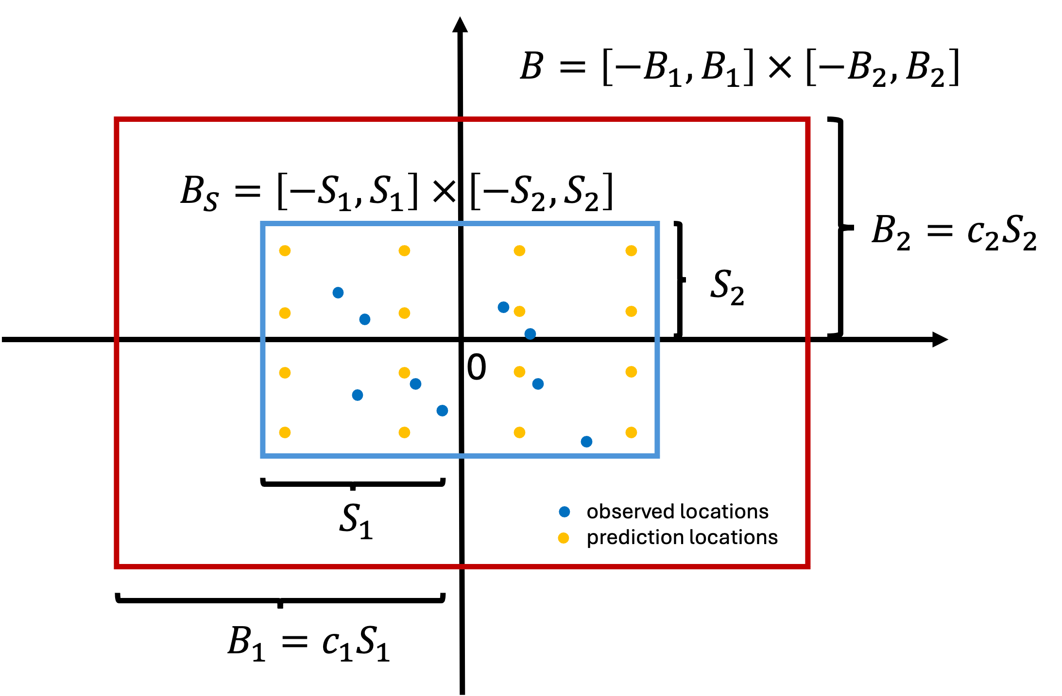
HSGP approximation box
- Due to the design of HSGP, the approximation is less accurate near the boundaries of \(B\).
- How much the approximation accuracy deteriorates towards the boundaries depends on smoothness of the true surface.
- The larger the length scale \(\rho\), the smoother the surface, a smaller box can be used for the same level of boundary accuracy.
- The larger the box, the more basis functions we need for the same level of overall accuracy, hence higher run time.
HSGP approximation box
- For ease of implementation, HSGP always centers all the coordinates.
- Let \(B_S\) denote the smallest box which contain all the observed and kriging locations. We need to ensure \(B_S \subset B\).
Relationship between \(c\), \(m\) and \(\rho\)
Let’s quickly recap. For simplicity, let \(d=1\),
- As \(\rho\) decreases, the surface is less smooth. \(c\) needs to increase to retain boundary accuracy.
- As \(c\) increases, \(m\) needs to increase to retain overall accuracy.
- As \(m\) increases, run time increases.
Riutort-Mayol et al. (2023) presented formulas for frequently used Matérn covariance functions:
- given \(\rho\), the minimum \(c\) and \(m\) needed
- given \(c\) and \(m\), the minimum \(\rho\) that can be captured
for a near 100% approximation accuracy of the correlation matrix.
However, \(\rho\) is unknown.
An iterative algorithm
Pseudo-codes for HSGP parameter tuning assuming \(d=1\).
HSGP implementation codes
Please clone the repo for AE 08 for HSGP implementation codes.
Side notes on HSGP implementation
A few random things to keep in mind for implementation in practice:
- If \(d>1\), parameter tuning is needed for each dimension.
- If your HSGP run is suspiciously VERY slow, check the number of basis functions being used in the run and make sure it is reasonable.
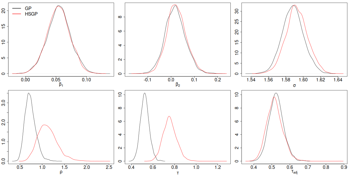
- Because HSGP is a low-rank approximation method, the GP magnitude parameter \(\tau\) will always be overestimated. However, we can account for this and use a bias-adjusted \(\tau\) instead. See AE 08
stancodes for parametertau_adj. - It is possible to use different length scale parameters for each dimension. See demo codes here for examples.
- The iterative algorithm described in Riutort-Mayol et al. (2023) (i.e., pseudo-codes on slide 12) can be further improved
- Due to identifiability issues, always look at \(\alpha \mathbf{1}+\boldsymbol{\theta}\) instead of \(\boldsymbol{\theta}\) alone.
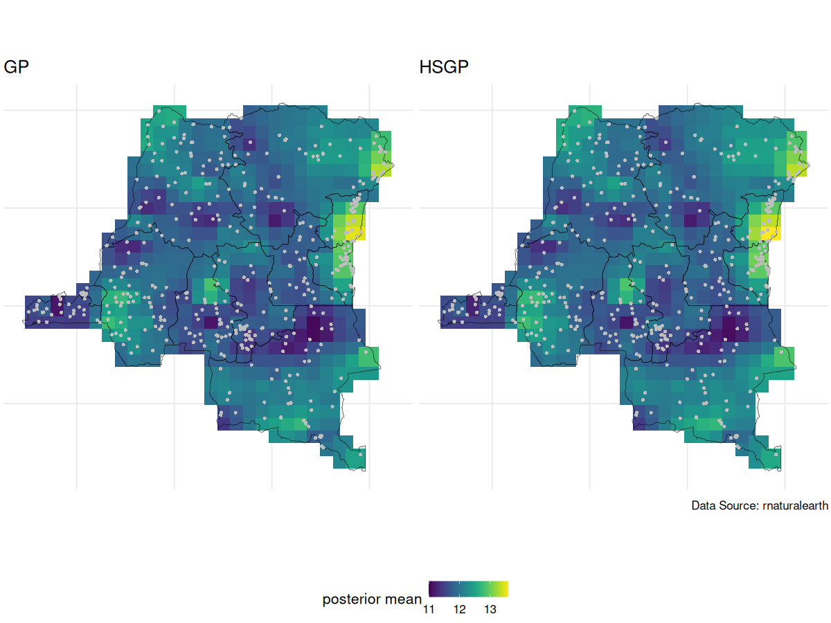
GP vs HSGP spatial intercept posterior mean
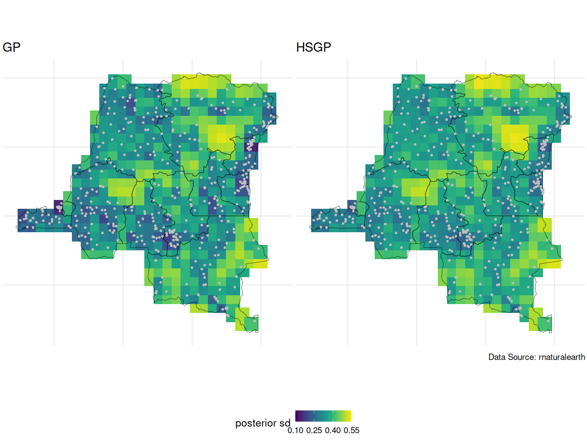
GP vs HSGP spatial intercept posterior SD
GP vs HSGP parameter posterior density
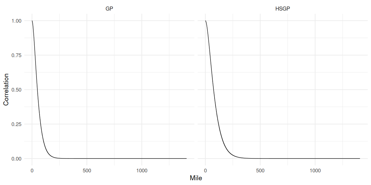
GP vs HSGP correlation function
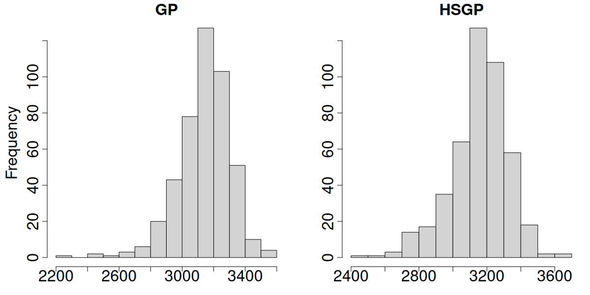
GP vs HSGP effective sample size
Prepare for next class
- Work on HW 05 which will be assigned shortly.
- Complete reading to prepare for Thursday’s lecture
- Thursday’s lecture: Disease Mapping
References
Riutort-Mayol, Gabriel, Paul-Christian Bürkner, Michael R Andersen, Arno Solin, and Aki Vehtari. 2023. “Practical Hilbert Space Approximate Bayesian Gaussian Processes for Probabilistic Programming.” Statistics and Computing 33 (1): 17.
Solin, Arno, and Simo Särkkä. 2020. “Hilbert Space Methods for Reduced-Rank Gaussian Process Regression.” Statistics and Computing 30 (2): 419–46.