Scalable Gaussian Processes #1

Christine Shen

Mar 19, 2026

Review of previous lectures

Over the past couple of weeks, we learned about:

1. Gaussian processes, and

2. How to use Gaussian processes for

   • longitudinal data
   • geospatial data

Motivating dataset

Recall we worked with a dataset on women aged 15-49 sampled from the 2013-14 Democratic Republic of Congo (DRC) Demographic and Health Survey. Variables are:

• loc_id: location id (i.e. survey cluster).

• hemoglobin: hemoglobin level (g/dL).

• anemia: anemia classifications.

• age: age in years.

• urban: urban vs. rural.

• LATNUM: latitude.

• LONGNUM: longitude.

Motivating dataset

  loc_id hemoglobin     anemia age urban   LATNUM  LONGNUM
1      1       12.5 not anemic  28 rural 0.220128 21.79508
2      1       12.6 not anemic  42 rural 0.220128 21.79508
3      1       13.3 not anemic  15 rural 0.220128 21.79508
4      1       12.9 not anemic  28 rural 0.220128 21.79508
5      1       10.4       mild  32 rural 0.220128 21.79508
6      1       12.2 not anemic  42 rural 0.220128 21.79508

Modeling goals:

• Learn the associations between age and urbanicity and hemoglobin, accounting for unmeasured spatial confounders.

• Create a predicted map of hemoglobin across the spatial surface controlling for age and urbanicity, with uncertainty quantification.

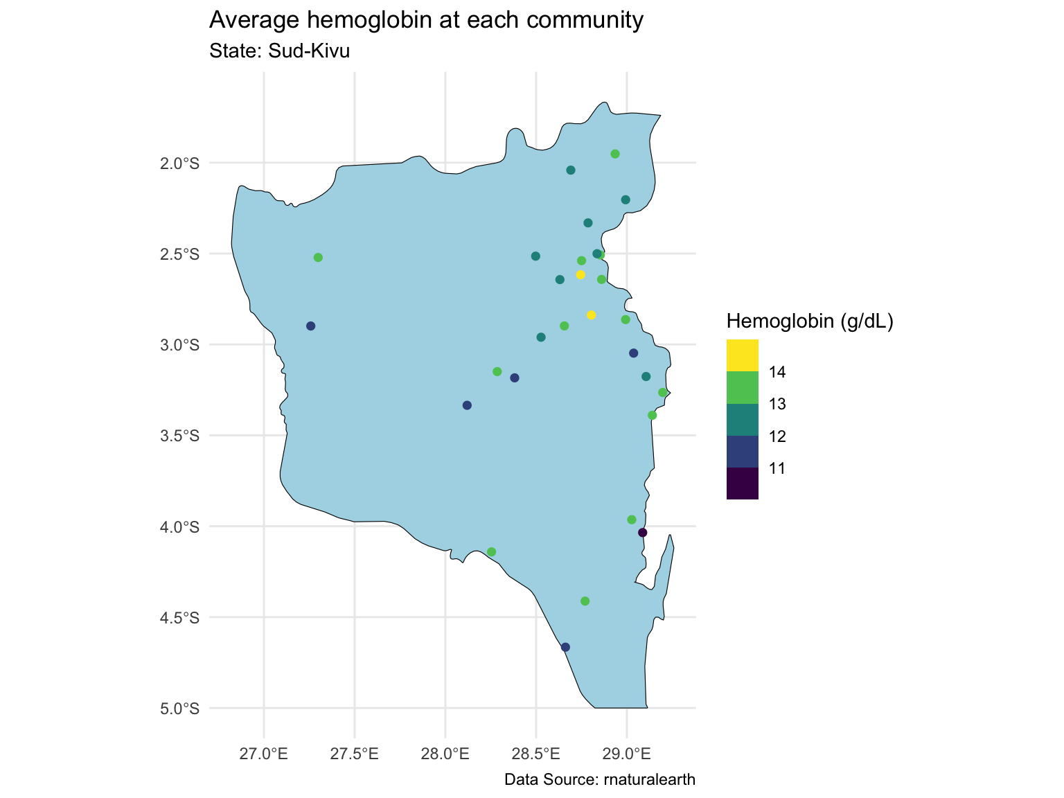
Map of the Sud-Kivu state

Last time, we focused on one state with ~500 observations at ~30 locations.

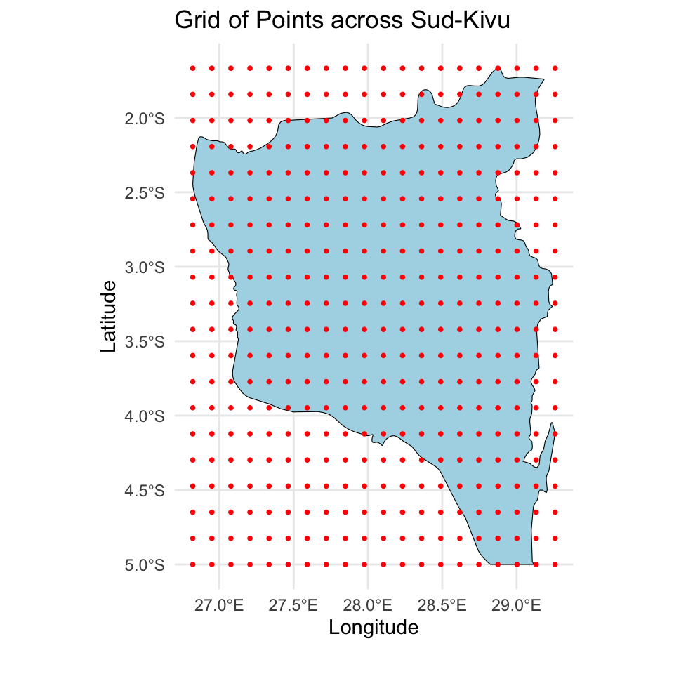
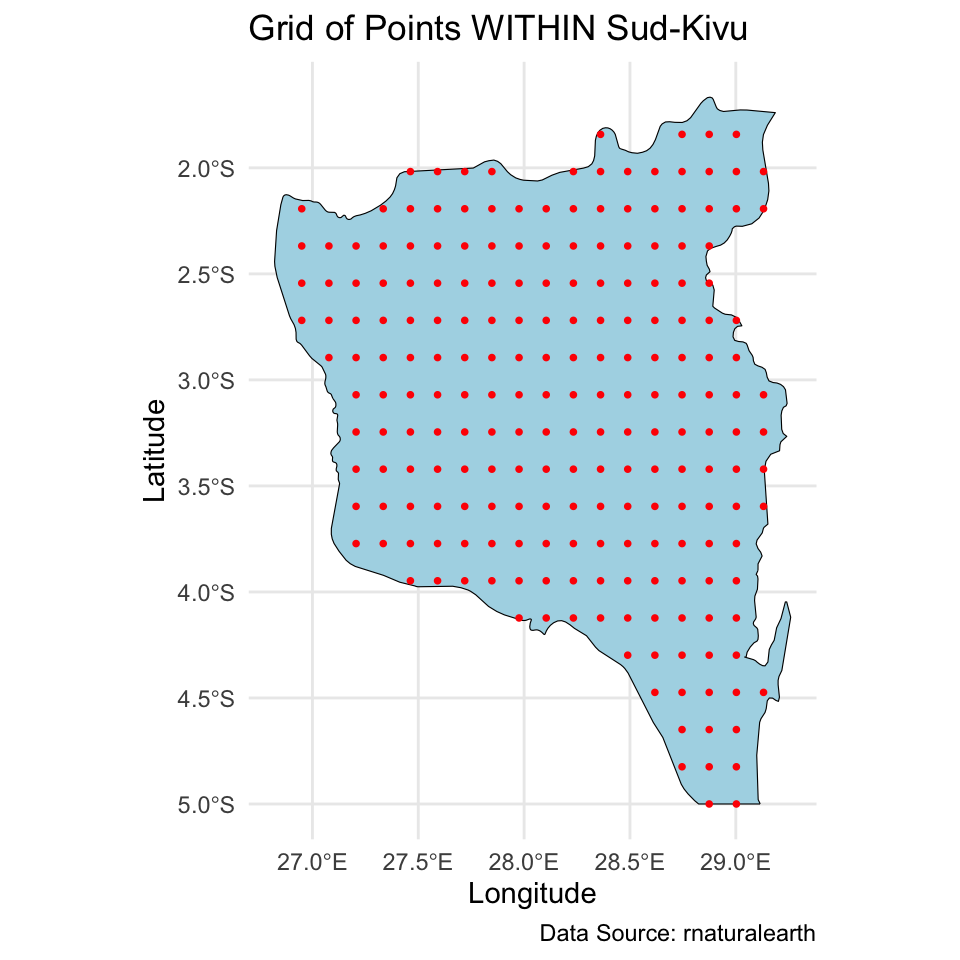
Prediction for the Sud-Kivu state

And we created a \(20 \times 20\) grid for prediction of the spatial intercept surface over the Sud-Kivu state.

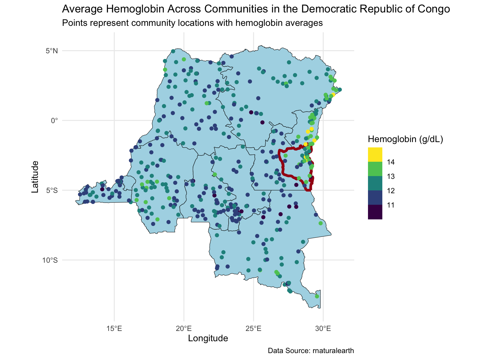
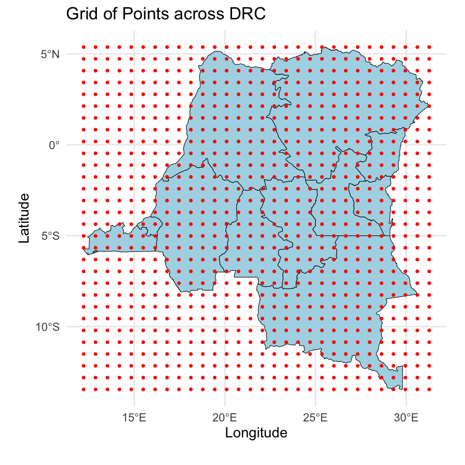
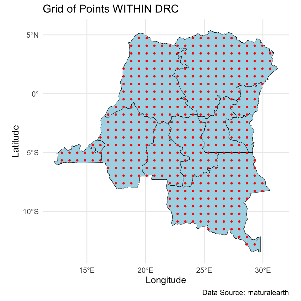
Map of the DRC

Today we will extend the analysis to the full dataset with ~8,600 observations at ~500 locations.

Prediction for the DRC

And we will make predictions on a \(30 \times 30\) grid over the DRC.

Modeling

\[\begin{align*} Y_j(\mathbf{u}_i) &= \alpha + \mathbf{x}_j(\mathbf{u}_i) \boldsymbol{\beta} + \theta(\mathbf{u}_i) + \epsilon_j(\mathbf{u}_i), \quad \epsilon_j(\mathbf{u}_i) \stackrel{iid}{\sim} N(0,\sigma^2) \end{align*}\]

Data objects:

• \(i \in \{1,\dots,n\}\) indexes unique locations.

• \(j \in \{1,\dots,n_i\}\) indexes individuals at each location.

• \(\mathbf{u}_i = (\text{longitude}_i,\text{latitude}_i) \in \mathbb{R}^2\) denotes coordinates of location \(i\).

• \(Y_j(\mathbf{u}_i)\) denotes the hemoglobin level of individual \(j\) at location \(\mathbf{u}_i\).

• \(\mathbf{x}_j(\mathbf{u}_i) = (\text{age}_{ij}/10,\text{urban}_i) \in \mathbb{R}^{1 \times p}\), where \(p=2\) is the number of predictors (excluding intercept).

Modeling

\[\begin{align*} Y_j(\mathbf{u}_i) &= \alpha + \mathbf{x}_j(\mathbf{u}_i) \boldsymbol{\beta} + \theta(\mathbf{u}_i) + \epsilon_j(\mathbf{u}_i), \quad \epsilon_j(\mathbf{u}_i) \stackrel{iid}{\sim} N(0,\sigma^2) \end{align*}\]

Population parameters:

• \(\alpha \in \mathbb{R}\) is the intercept.

• \(\boldsymbol{\beta} \in \mathbb{R}^p\) is the regression coefficients.

• \(\sigma^2 \in \mathbb{R}^+\) is the overall residual error (nugget).

Location-specific parameters:

• \(\theta(\mathbf{u}_i)\) denotes the spatial intercept at location \(\mathbf{u}_i\).

Location-specific notation

\[\mathbf{Y}(\mathbf{u}_i) = \alpha \mathbf{1}_{n_i} + \mathbf{X}(\mathbf{u}_i) \boldsymbol{\beta} + \theta(\mathbf{u}_i)\mathbf{1}_{n_i} + \boldsymbol{\epsilon}(\mathbf{u}_i), \quad \boldsymbol{\epsilon}(\mathbf{u}_i) \sim N_{n_i}(\mathbf{0},\sigma^2\mathbf{I})\]

• \(\mathbf{Y}(\mathbf{u}_i) = (Y_1(\mathbf{u}_i),\ldots,Y_{n_i}(\mathbf{u}_i))^\top\).

• \(\mathbf{X}(\mathbf{u}_i)\) is an \(n_i \times p\) dimensional matrix with rows \(\mathbf{x}_j(\mathbf{u}_i)\).

• \(\boldsymbol{\epsilon}(\mathbf{u}_i) = (\epsilon_i(\mathbf{u}_i),\ldots,\epsilon_{n_i}(\mathbf{u}_i))^\top\).

Full data notation

\[\mathbf{Y} = \alpha \mathbf{1}_{N} + \mathbf{X} \boldsymbol{\beta} + \mathbf{Z}\boldsymbol{\theta} + \boldsymbol{\epsilon}, \quad \boldsymbol{\epsilon} \sim N_N(\mathbf{0},\sigma^2\mathbf{I})\]

• \(\mathbf{Y} = (\mathbf{Y}(\mathbf{u}_1)^\top,\ldots,\mathbf{Y}(\mathbf{u}_{n})^\top)^\top \in \mathbb{R}^N\), with \(N = \sum_{i=1}^n n_i\).

• \(\mathbf{X} \in \mathbb{R}^{N \times p}\) stacks \(\mathbf{X}(\mathbf{u}_i)\).

• \(\boldsymbol{\theta} = (\theta(\mathbf{u}_1),\ldots,\theta(\mathbf{u}_n))^\top \in \mathbb{R}^n\).

• \(\mathbf{Z}\) is an \(N \times n\) dimensional block diagonal binary matrix. Each row contains a single 1 in column \(i\) that corresponds to the location of \(Y_j(\mathbf{u}_i)\). \[ \begin{align} \mathbf{Z} = \begin{bmatrix} \mathbf{1}_{n_1} & \mathbf{0} & \dots & \mathbf{0} \\ \mathbf{0} & \mathbf{1}_{n_2} & \dots & \mathbf{0} \\ \vdots & \vdots & \ddots & \vdots \\ \mathbf{0} & \dots & \mathbf{0} & \mathbf{1}_{n_n} \end{bmatrix}. \end{align} \]

Modeling

We specify the following model: \[\mathbf{Y} = \alpha \mathbf{1}_{N} + \mathbf{X} \boldsymbol{\beta} + \mathbf{Z}\boldsymbol{\theta} + \boldsymbol{\epsilon}, \quad \boldsymbol{\epsilon} \sim N_N(\mathbf{0},\sigma^2\mathbf{I})\] with priors

• \(\boldsymbol{\theta}(\mathbf{u}) | \tau,\rho \sim GP(\mathbf{0},C(\cdot,\cdot))\), where \(C\) is the Matérn 3/2 covariance function with magnitude \(\tau\) and length scale \(\rho\).
• \(\alpha^* \sim N(0,4^2)\). This is the intercept after centering \(\mathbf{X}\).
• \(\beta_j | \sigma_{\beta} \sim N(0,\sigma_{\beta}^2)\), \(j \in \{1,\dots,p\}\)
• \(\sigma \sim \text{Half-Normal}(0, 2^2)\)
• \(\tau \sim \text{Half-Normal}(0, 4^2)\)
• \(\rho \sim \text{Inv-Gamma}(5, 5)\)
• \(\sigma_{\beta} \sim \text{Half-Normal}(0, 2^2)\)

Computational issues with GP

Effectively, the prior for \(\boldsymbol{\theta}\) is \[\boldsymbol{\theta} | \tau,\rho \sim N_n(\mathbf{0},\mathbf{C}), \quad \mathbf{C} \in \mathbb{R}^{n \times n}.\] Matérn 3/2 is an isotropic covariance function, \(C(\mathbf{u}_i, \mathbf{u}_j) = C(\|\mathbf{u}_i-\mathbf{u}_j\|)\).

\[\mathbf{C} = \begin{bmatrix} C(\mathbf{0}) & C(\|\mathbf{u}_1 - \mathbf{u}_2\|) & \cdots & C(\|\mathbf{u}_1 - \mathbf{u}_n\|)\\ C(\|\mathbf{u}_1 - \mathbf{u}_2\|) & C(\mathbf{0}) & \cdots & C(\|\mathbf{u}_2 - \mathbf{u}_n\|)\\ \vdots & \vdots & \ddots & \vdots\\ C(\|\mathbf{u}_{1} - \mathbf{u}_n\|) & C(\|\mathbf{u}_2 - \mathbf{u}_n\|) & \cdots & C(\mathbf{0})\\ \end{bmatrix}.\]

This is not scalable because we need to invert an \(n \times n\) dense covariance matrix for each MCMC iteration, which requires \(\mathcal{O}(n^3)\) floating point operations (flops), and \(\mathcal{O}(n^2)\) memory.

Scalable GP methods overview

The computational issues motivated exploration in scalable GP methods. Existing scalable methods broadly fall under two categories.

1. Sparsity methods

   • sparsity in \(\mathbf{C}\), e.g., covariance tapering (Furrer, Genton, and Nychka (2006)).
   • sparsity in \(\mathbf{C}^{-1}\), e.g., Vecchia approximation (Vecchia (1988)) and nearest-neighbor GP (Datta et al. (2016)).

2. Low-rank methods

   • approximate \(\mathbf{C}\) on a low-dimensional subspace.
   • e.g., process convolution (Higdon (2002)), inducing point method(Snelson and Ghahramani (2005)).

Hilbert space method for GP

• Solin and Särkkä (2020) introduced a Hilbert space method for reduced-rank Gaussian process regression (HSGP).

• Riutort-Mayol et al. (2023) discussed how to practically implement HSGP.

• Tutorial codes are available in different probabilistic programming languages:

  • stan
  • NumPyro
  • pyMC

Lecture plan

Today:

• How does HSGP work
• Why HSGP is scalable
• How to use HSGP for Bayesian geospatial model fitting
• How to use HSGP for posterior predictive sampling

Next Tuesday:

• How to use HSGP for posterior predictive sampling
• Parameter tuning for HSGP
• How to implement HSGP in stan

HSGP approximation

Given:

• an isotropic covariance function \(C\) which admits a power spectral density, e.g., the Matérn family, and
• a compact domain \(B \in \mathbb{R}^d\) with nice boundaries. For our purposes, we only consider boxes, e.g., \([-1,1] \times [-1,1]\).

HSGP approximates the \((i,j)\) element of the corresponding \(n \times n\) covariance matrix \(\mathbf{C}\) as \[\mathbf{C}_{ij}=C(\|\mathbf{u}_i - \mathbf{u}_j\|) \approx \sum_{k=1}^m s_k(\tau,\rho)\phi_k(\mathbf{u}_i)\phi_k(\mathbf{u}_j).\]

HSGP approximation

\[\mathbf{C}_{ij}=C(\|\mathbf{u}_i - \mathbf{u}_j\|) \approx \sum_{k=1}^m s_k(\tau,\rho)\phi_k(\mathbf{u}_i)\phi_k(\mathbf{u}_j).\]

• \(s_k \in \mathbb{R}^+\) are positive scalars which depends on the covariance function \(C\) and its parameters \(\tau\) and \(\rho\).
• \(\phi_k: B \to \mathbb{R}\) are basis functions which only depends on \(B\).
• \(m\) is the number of basis functions. Note: even with an infinite sum (i.e., \(m \to \infty\)), this remains an approximation (see Solin and Särkkä (2020)).

HSGP approximation

In matrix notation,

\[\mathbf{C} \approx \boldsymbol{\Phi} \mathbf{S} \boldsymbol{\Phi}^\top.\]

• \(\boldsymbol{\Phi} \in \mathbb{R}^{n \times m}\) is a feature matrix. Only depends on \(B\) and the observed locations.
• \(\mathbf{S} \in \mathbb{R}^{m \times m}\) is diagonal. Depends on the covariance function \(C\) and parameters \(\tau\) and \(\rho\).

\[ \begin{align} \boldsymbol{\Phi} = \begin{bmatrix} \phi_1(\mathbf{u}_1) & \dots & \phi_m(\mathbf{u}_1) \\ \vdots & \ddots & \vdots \\ \phi_1(\mathbf{u}_n) & \dots & \phi_m(\mathbf{u}_n) \end{bmatrix}, \quad \mathbf{S} = \begin{bmatrix} s_1 & & \\ & \ddots & \\ & & s_m \end{bmatrix}. \end{align} \]

Model reparameterization

Under HSGP approximation, \[\boldsymbol{\theta} \overset{d}{=} \boldsymbol{\Phi} \mathbf{S}^{1/2}\mathbf{b}, \quad \mathbf{b} \sim N_m(0,\mathbf{I}).\]

Therefore we can reparameterize the model as

\[ \begin{align} \mathbf{Y} &= \alpha \mathbf{1}_{N} + X\boldsymbol{\beta} + \mathbf{Z}\boldsymbol{\theta} + \boldsymbol{\epsilon} \\ &\approx \alpha \mathbf{1}_{N} + X\boldsymbol{\beta} + \underbrace{\mathbf{Z}\boldsymbol{\Phi} \mathbf{S}^{1/2}}_{\mathbf{W}}\mathbf{b} + \boldsymbol{\epsilon} \end{align} \]

Note the resemblance to linear regression:

• \(\mathbf{W} \in \mathbb{R}^{n \times m}\) is a known design matrix given parameters \(\tau\) and \(\rho\).
• \(\mathbf{b}\) is an unknown parameter vector with prior \(N_m(0,\mathbf{I})\).

Why HSGP is scalable

HSGP approximation in matrix form:

\[\mathbf{C} \approx \boldsymbol{\Phi} \mathbf{S} \boldsymbol{\Phi}^\top.\]

• No matrix inversion.

• \(\boldsymbol{\Phi}\) only depends on \(B\) and the observed locations, can be pre-calculated.

• Each MCMC iteration requires \(\mathcal{O}(nm + m)\) flops, vs \(\mathcal{O}(n^3)\) for a full GP.

• Ideally \(m \ll n\), but HSGP can be faster even for \(m>n\).

HSGP in stan

We can implement the reparameterized model in stan. See pseudocodes below. This is called the non-centered parameterization in stan documentation. It’s recommended for computational efficiency for hierarchical models.

data{
  matrix[N,m] Z;
  matrix[N,p] X;
  matrix[n,2] u; // locations for observed data
  ...
}
transformed data {
  matrix[n,m] PHI;
  matrix[N,p] X_centered;
  ...
}
parameters {
  real alpha_star;
  real<lower=0> sigma;
  vector[p] beta;
  vector[m] b;
  vector<lower=0>[m] sqrt_S;
  ...
}
model {
  vector[n] theta = PHI * (sqrt_S .* b);
  target += normal_lupdf(y | alpha_star + X_centered * beta + Z * theta, sigma);
  target += normal_lupdf(b | 0, 1);
  ...
}

Posterior predictive distribution

We want to make predictions for \(\mathbf{Y}^* = (Y(\mathbf{u}_{n+1}),\ldots, Y(\mathbf{u}_{n+q}))^\top\), observations at \(q\) new locations. Define \(\boldsymbol{\theta}^* = (\theta(\mathbf{u}_{n+1}),\ldots,\theta(\mathbf{u}_{n+q}))^\top\), \(\boldsymbol{\Omega} = (\alpha,\boldsymbol{\beta},\sigma,\tau,\rho)\). Recall:

\[\begin{align*} f(\mathbf{Y}^* | \mathbf{Y}) &= \int f(\mathbf{Y}^*, \boldsymbol{\theta}^*, \boldsymbol{\theta}, \boldsymbol{\Omega} | \mathbf{Y}) d\boldsymbol{\theta}^* d\boldsymbol{\theta} d\boldsymbol{\Omega}\\ &= \int \underbrace{f(\mathbf{Y}^* | \boldsymbol{\theta}^*, \boldsymbol{\Omega})}_{(1)} \underbrace{f(\boldsymbol{\theta}^* | \boldsymbol{\theta}, \boldsymbol{\Omega})}_{(2)} \underbrace{f(\boldsymbol{\theta},\boldsymbol{\Omega} | \mathbf{Y})}_{(3)} d\boldsymbol{\theta}^* d\boldsymbol{\theta} d\boldsymbol{\Omega}\\ \end{align*}\]

1. Likelihood: \(f(\mathbf{Y}^* | \boldsymbol{\theta}^*, \boldsymbol{\Omega})\) – remains the same as for GP

2. Kriging: \(f(\boldsymbol{\theta}^* | \boldsymbol{\theta}, \boldsymbol{\Omega})\) – we will focus on this next

3. Posterior distribution: \(f(\boldsymbol{\theta},\boldsymbol{\Omega} | \mathbf{Y})\) – we have just discussed

Kriging

Recall under the GP prior,

\[\begin{bmatrix} \boldsymbol{\theta}\\ \boldsymbol{\theta}^* \end{bmatrix} \Bigg| \boldsymbol{\Omega} \sim N_{n+q}\left(\begin{bmatrix} \mathbf{0}_n \\ \mathbf{0}_q \end{bmatrix}, \begin{bmatrix} \mathbf{C} & \mathbf{C}_{+}\\ \mathbf{C}_{+}^\top & \mathbf{C}^* \end{bmatrix}\right),\]

where \(\mathbf{C}\) is the covariance of \(\boldsymbol{\theta}\), \(\mathbf{C}^*\) is the covariance of \(\boldsymbol{\theta}^*\), and \(\mathbf{C}_{+}\) is the cross covariance matrix between \(\boldsymbol{\theta}\) and \(\boldsymbol{\theta}^*\).

Therefore by properties of multivariate normal, \[\boldsymbol{\theta}^* \mid (\boldsymbol{\theta}, \boldsymbol{\Omega}) \sim N_q(\mathbb{E}_{\boldsymbol{\theta}^*},\mathbb{V}_{\boldsymbol{\theta}^*}), \quad \text{where}\] \[ \begin{align} \mathbb{E}_{\boldsymbol{\theta}^*} &= \mathbf{C}_+^\top \mathbf{C}^{-1} \boldsymbol{\theta}\\ \mathbb{V}_{\boldsymbol{\theta}^*} &= \mathbf{C}^* - \mathbf{C}_+^\top \mathbf{C}^{-1} \mathbf{C}_+. \end{align} \]

Kriging under HSGP

Under HSGP, \(\mathbf{C}^* \approx \boldsymbol{\Phi}^* \mathbf{S}\boldsymbol{\Phi}^{*\top}\), \(\mathbf{C}_+ \approx \boldsymbol{\Phi} \mathbf{S}\boldsymbol{\Phi}^{*\top}\), where \[ \begin{align} \boldsymbol{\Phi}^* \in \mathbb{R}^{q \times m} = \begin{bmatrix} \phi_1(\mathbf{u}_{n+1}) & \dots & \phi_m(\mathbf{u}_{n+1}) \\ \vdots & \ddots & \vdots \\ \phi_1(\mathbf{u}_{n+q}) & \dots & \phi_m(\mathbf{u}_{n+q}) \end{bmatrix} \end{align} \] is the feature matrix for the new locations. Therefore approximately \[\begin{align} \begin{bmatrix} \boldsymbol{\theta} \\ \boldsymbol{\theta}^* \end{bmatrix} \Bigg| \boldsymbol{\Omega} \sim N_{n +q} \left(\begin{bmatrix} \mathbf{0}_n \\ \mathbf{0}_q \end{bmatrix}, \begin{bmatrix} \boldsymbol{\Phi}\mathbf{S}\boldsymbol{\Phi}^\top & \boldsymbol{\Phi}\mathbf{S} \boldsymbol{\Phi}^{*\top} \\ \boldsymbol{\Phi}^*\mathbf{S}\boldsymbol{\Phi}^\top & \boldsymbol{\Phi}^*\mathbf{S}\boldsymbol{\Phi}^{*\top} \end{bmatrix} \right). \end{align} \]

Kriging under HSGP

Under the reparameterized model, it is easy to recognize the kriging distribution under HSGP.

Recall we model \(\boldsymbol{\theta} = \boldsymbol{\Phi} \mathbf{S}^{1/2}\mathbf{b}\), where \(\mathbf{b}\) is treated as the unknown parameter, and \(S\) is known given \(\tau\) and \(\rho\). Therefore for kriging:

\[\begin{align} \boldsymbol{\theta}^* \mid (\boldsymbol{\theta},\boldsymbol{\Omega}) &= \boldsymbol{\Phi}^*\mathbf{S}^{1/2}\mathbf{b} \mid (\mathbf{b},\boldsymbol{\Omega}) \\ &=\boldsymbol{\Phi}^*\mathbf{S}^{1/2}\mathbf{b}. \end{align}\]

During MCMC sampling, we can obtain posterior predictive samples for \(\boldsymbol{\theta}^*\) through posterior samples of \(\mathbf{b}\) and \(\mathbf{S}\). Let superscript \((s)\) denote the \(s\)th posterior sample:

\[\boldsymbol{\theta}^{*(s)} = \boldsymbol{\Phi}^* \mathbf{S}^{(s) 1/2} \mathbf{b}^{(s)}.\]

HSGP kriging in stan

Under HSGP, kriging can be easily implemented in stan.

data {
  matrix[n,2] u_new; // locations for prediction
  ...
}
transformed data {
  matrix[q,m] PHI_new;
  ...
}
parameters {
  vector[m] b;
  vector<lower=0>[m] sqrt_S;
  ...
}
model {
  ...
}
generated quantities {
  vector[q] theta_new = PHI_new * (sqrt_S .* b);
}

Kriging under HSGP

We mathematically show the kriging results. Recall under HSGP: \[\begin{align} \begin{bmatrix} \boldsymbol{\theta} \\ \boldsymbol{\theta}^* \end{bmatrix} \Bigg| \boldsymbol{\Omega} \sim N_{n +q} \left(\begin{bmatrix} \mathbf{0}_n \\ \mathbf{0}_q \end{bmatrix}, \begin{bmatrix} \boldsymbol{\Phi}\mathbf{S}\boldsymbol{\Phi}^\top & \boldsymbol{\Phi}\mathbf{S} \boldsymbol{\Phi}^{*\top} \\ \boldsymbol{\Phi}^*\mathbf{S}\boldsymbol{\Phi}^\top & \boldsymbol{\Phi}^*\mathbf{S}\boldsymbol{\Phi}^{*\top} \end{bmatrix} \right). \end{align} \]

Again by properties of multivariate normal, \[\boldsymbol{\theta}^* \mid (\boldsymbol{\theta}, \boldsymbol{\Omega}) \overset{?}{\sim} N_q(\mathbb{E}_{\boldsymbol{\theta}^*}^{HS},\mathbb{V}_{\boldsymbol{\theta}^*}^{HS}),\]

\[ \begin{align} \mathbb{E}_{\boldsymbol{\theta}^*}^{HS} &= (\boldsymbol{\Phi}^*\mathbf{S}\boldsymbol{\Phi}^\top) (\boldsymbol{\Phi}\mathbf{S}\boldsymbol{\Phi}^\top)^{-1} \boldsymbol{\theta}\\ \mathbb{V}_{\boldsymbol{\theta}^*}^{HS} &= (\boldsymbol{\Phi}^*\mathbf{S}\boldsymbol{\Phi}^{*\top}) - (\boldsymbol{\Phi}^*\mathbf{S}\boldsymbol{\Phi}^\top) (\boldsymbol{\Phi}\mathbf{S}\boldsymbol{\Phi}^\top)^{-1}(\boldsymbol{\Phi}\mathbf{S} \boldsymbol{\Phi}^{*\top}). \end{align} \]

• If \(m \ge n\), \((\boldsymbol{\Phi}\mathbf{S}\boldsymbol{\Phi}^\top)\) is invertible, and this is the kriging distribution.
• But what if \(m < n\)?

Kriging under HSGP

If \(m \le n\), claim \(\boldsymbol{\theta}^* \mid (\boldsymbol{\theta}, \boldsymbol{\Omega}) = (\boldsymbol{\Phi}^*\mathbf{S}\boldsymbol{\Phi}^\top) (\boldsymbol{\Phi}\mathbf{S}\boldsymbol{\Phi}^\top)^{\dagger} \boldsymbol{\theta},\) where \(\mathbf{A}^\dagger\) denotes a generalized inverse of matrix \(\mathbf{A}\) such that \(\mathbf{A}\mathbf{A}^{\dagger}\mathbf{A} = \mathbf{A}\). Sketch proof below, see details in class.

1. By properties of multivariate normal, \(\boldsymbol{\theta}^* \mid (\boldsymbol{\theta}, \boldsymbol{\Omega}) \sim N_q(\mathbb{E}_{\boldsymbol{\theta}^*}^{HS},\mathbb{V}_{\boldsymbol{\theta}^*}^{HS})\), \[ \begin{align} \mathbb{E}_{\boldsymbol{\theta}^*}^{HS} &= (\boldsymbol{\Phi}^*\mathbf{S}\boldsymbol{\Phi}^\top) (\boldsymbol{\Phi}\mathbf{S}\boldsymbol{\Phi}^\top)^{\dagger} \boldsymbol{\theta}\\ \mathbb{V}_{\boldsymbol{\theta}^*}^{HS} &= (\boldsymbol{\Phi}^*\mathbf{S}\boldsymbol{\Phi}^{*\top}) - (\boldsymbol{\Phi}^*\mathbf{S}\boldsymbol{\Phi}^\top) (\boldsymbol{\Phi}\mathbf{S}\boldsymbol{\Phi}^\top)^{\dagger \top}(\boldsymbol{\Phi}\mathbf{S} \boldsymbol{\Phi}^{*\top}). \end{align} \]

2. Show if \(\boldsymbol{\Phi}\) has full column rank, which is true under HSGP, then \[ \begin{align} \mathbf{S} \boldsymbol{\Phi}^\top(\boldsymbol{\Phi}\mathbf{S}\boldsymbol{\Phi}^\top)^{\dagger \top}\boldsymbol{\Phi}\mathbf{S} = \mathbf{S} \tag{1} \\ \mathbf{S} \boldsymbol{\Phi}^\top(\boldsymbol{\Phi}\mathbf{S}\boldsymbol{\Phi}^\top)^{\dagger}\boldsymbol{\Phi}\mathbf{S} = \mathbf{S} \tag{2}. \end{align} \] Equation (1) is sufficient to show \(\mathbb{V}_{\boldsymbol{\theta}^*}^{HS} \equiv \mathbf{0}\).

Kriging under HSGP

Under the reparameterized model, \(\boldsymbol{\theta} = \boldsymbol{\Phi} \mathbf{S}^{1/2}\mathbf{b}\), for \(\mathbf{b} \sim N_m(0,\mathbf{I}).\) Therefore \[ \begin{align} \boldsymbol{\theta}^* \mid (\boldsymbol{\theta},\boldsymbol{\Omega}) &= (\boldsymbol{\Phi}^*\mathbf{S}\boldsymbol{\Phi}^\top) (\boldsymbol{\Phi}\mathbf{S}\boldsymbol{\Phi}^\top)^{\dagger} \boldsymbol{\theta} \\ &= (\boldsymbol{\Phi}^*\mathbf{S}\boldsymbol{\Phi}^\top) (\boldsymbol{\Phi}\mathbf{S}\boldsymbol{\Phi}^\top)^{\dagger}(\boldsymbol{\Phi} \mathbf{S}^{1/2}\mathbf{b}) \\ &= \boldsymbol{\Phi}^*\mathbf{S}^{1/2}\mathbf{b}. \quad (\text{by equation (2) in the last slide}) \end{align} \]

Next class, we will look at situations where \(m>n\).

Recap

HSGP is a low rank approximation method for GP.

\[\begin{align} \mathbf{C}_{ij} \approx \sum_{k=1}^m s_k\phi_k(\mathbf{u}_i)\phi_k(\mathbf{u}_j), \quad \mathbf{C} \approx \boldsymbol{\Phi} \mathbf{S} \boldsymbol{\Phi}^\top, \end{align}\]

• for covariance function \(C\) which admits a power spectral density, on a box \(B \subset \mathbb{R}^d\).
• with \(m\) number of basis functions.

We have talked about:

• why HSGP is scalable.
• how to do posterior sampling in stan.
• how to do posterior predictive sampling in stan if \(m \le n\).

Prepare for next class

1. Work on HW 04 which is due before class next Tuesday.

2. Complete reading to prepare for Tuesday’s lecture

3. Tuesday’s lecture:

   • How to posterior predictive sampling in stan if \(m > n\)
   • Parameter tuning for HSGP
   • How to implement HSGP in stan

References

Datta, Abhirup, Sudipto Banerjee, Andrew O Finley, and Alan E Gelfand. 2016. “Hierarchical Nearest-Neighbor Gaussian Process Models for Large Geostatistical Datasets.” Journal of the American Statistical Association 111 (514): 800–812.

Furrer, Reinhard, Marc G Genton, and Douglas Nychka. 2006. “Covariance Tapering for Interpolation of Large Spatial Datasets.” Journal of Computational and Graphical Statistics 15 (3): 502–23.

Higdon, Dave. 2002. “Space and Space-Time Modeling Using Process Convolutions.” In Quantitative Methods for Current Environmental Issues, 37–56. Springer.

Riutort-Mayol, Gabriel, Paul-Christian Bürkner, Michael R Andersen, Arno Solin, and Aki Vehtari. 2023. “Practical Hilbert Space Approximate Bayesian Gaussian Processes for Probabilistic Programming.” Statistics and Computing 33 (1): 17.

Snelson, Edward, and Zoubin Ghahramani. 2005. “Sparse Gaussian Processes Using Pseudo-Inputs.” Advances in Neural Information Processing Systems 18.

Solin, Arno, and Simo Särkkä. 2020. “Hilbert Space Methods for Reduced-Rank Gaussian Process Regression.” Statistics and Computing 30 (2): 419–46.

Vecchia, Aldo V. 1988. “Estimation and Model Identification for Continuous Spatial Processes.” Journal of the Royal Statistical Society Series B: Statistical Methodology 50 (2): 297–312.