    weight   height  sex
1 144.6231 68.50397 Male
2 158.2917 69.01579 Male
3 177.9128 76.18114 Male
4 160.0554 73.42524 Male
5 173.7241 73.70083 Male
6 164.9056 71.45673 MaleBayesian Workflow
Prof. Sam Berchuck
Feb 03, 2026
Review of last lecture
On Thursday, we learned about various ways compare models.
AIC, DIC, WAIC
LOO-CV/LOO-IC
Today, we will put these concepts within the larger framework of the Bayesian workflow.
Bayes theorem
\[f(\boldsymbol{\theta} | \mathbf{Y}) = \frac{f(\mathbf{Y} | \boldsymbol{\theta})f(\boldsymbol{\theta})}{f(\mathbf{Y})}\]
- Rethinking Bayes theorem:
\[f(\boldsymbol{\theta} | \mathbf{Y}) \propto f(\mathbf{Y}, \boldsymbol{\theta}) = f(\mathbf{Y} | \boldsymbol{\theta})f(\boldsymbol{\theta}) \]
- In Stan:
\[\log f(\mathbf{Y} | \boldsymbol{\theta}) + \log f(\boldsymbol{\theta})\]
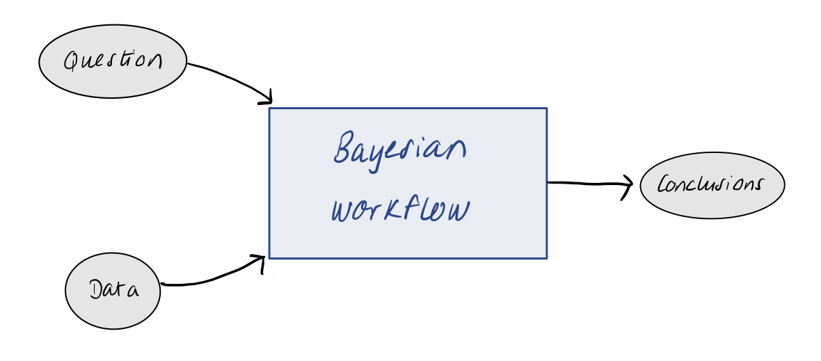
Bayesian workflow
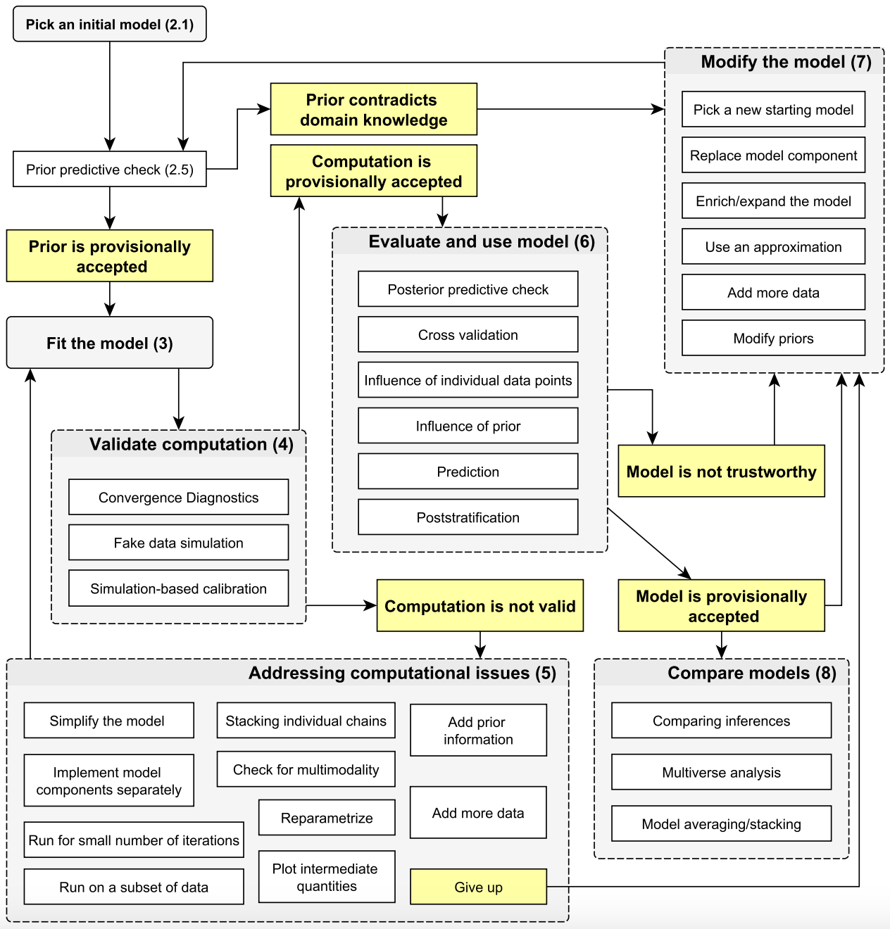
Bayesian workflow
- Today we will talk about a general strategy for taking a question and data to a robust conclusion.
A simplified workflow
Setting up a full probability model: a joint probability distribution for all observable and unobservable quantities in a problem. The model should be consistent with knowledge about the underlying scientific problem and the data collection process.
Conditioning on observed data: calculating and interpreting the appropriate posterior distribution — the conditional probability distribution of the unobserved quantities of ultimate interest, given the observed data.
Evaluating the fit of the model and the implications of the resulting posterior distribution: how well does the model fit the data, are the substantive conclusions reasonable, and how sensitive are the results to the modeling assumptions in step 1? In response, one can alter or expand the model and repeat the three steps.
From BDA3.
Bayesian workflow
- Research question: What are your dependent and indepednent variables? What associations are you interested in? EDA.
- Specify likelihood & priors: Use knowledge of the problem to construct a generative model.
- Check the model with simulated data: Generate data from the model and evaluate fit as a sanity check (prior predictive checks).
- Fit the model to real data: Estimate parameters using MCMC.
Bayesian workflow
- Check diagnostics: Use MCMC diagnostics to guarentee that the algorithm converged.
- Examine posterior fit: Create posterior summaries that are relevant to the research question.
- Check predictions: Examing posterior predictive checks.
- Compare models: Iterate on model design and choose a model.
Motivating example: predicting weight from height
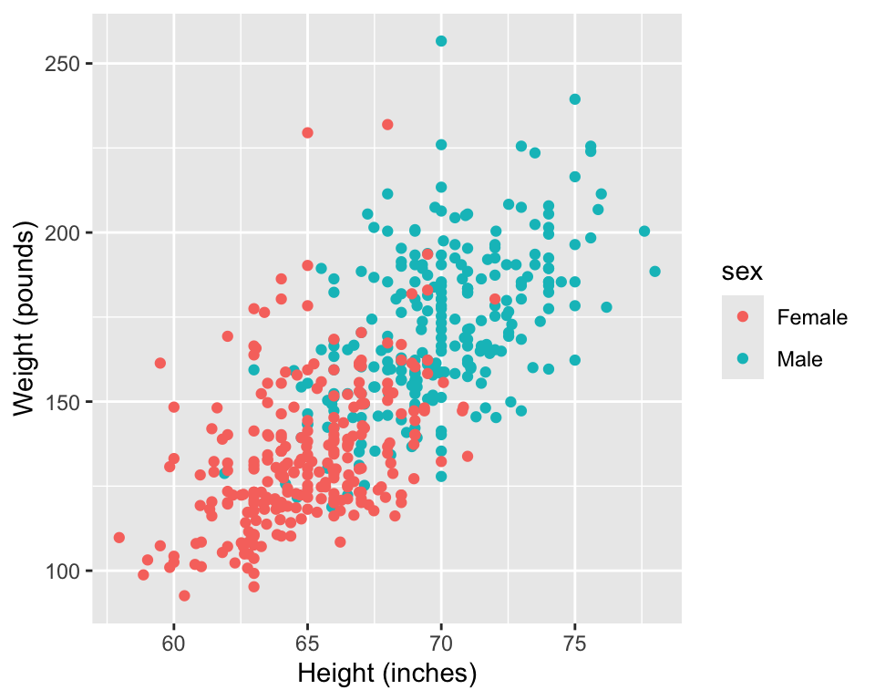
Research question: We would like to understand the relationship between a person’s height and weight. A few particular questions we have are:
How much does a person’s weight increase when their height increases?
How certain can we be about the magnitude of the increase?
Can we predict a person’s weight based on their height?
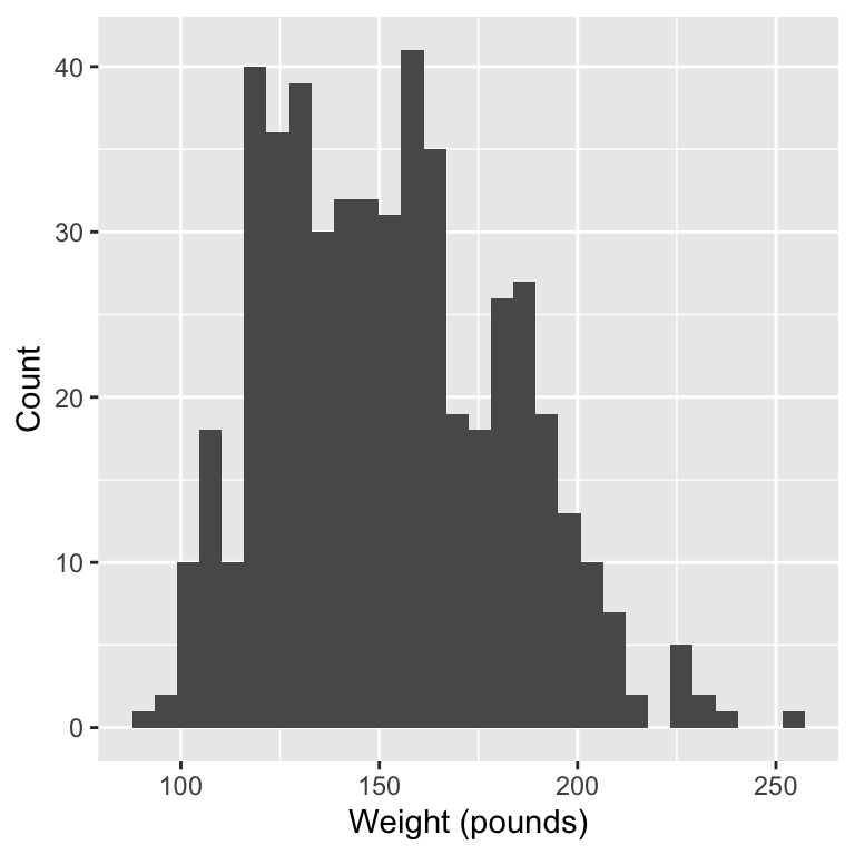
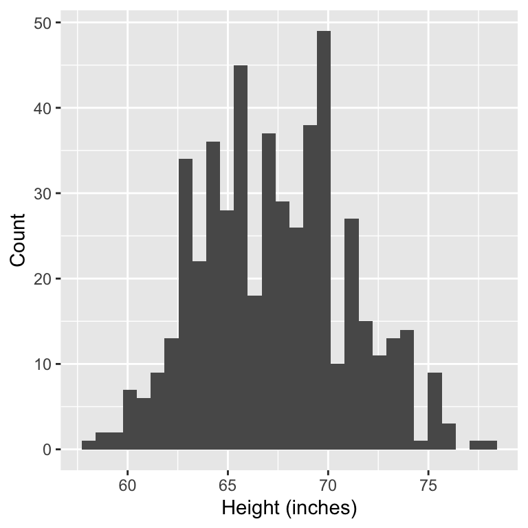
Data: We will use the bdims dataset from the openintro package. This dataset contains body girth measurements and skeletal diameter measurements, as well as age, weight, height and gender.
Prepare data
1. Research question:
1. Research question:
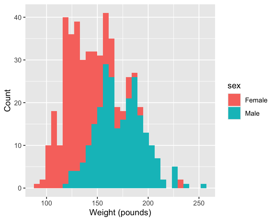
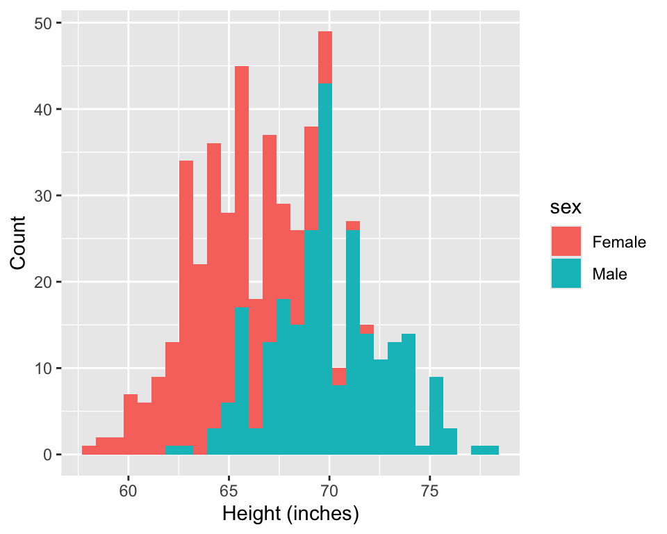
1. Research question:
2. Specify likelihood & priors:
Construct a data generating process.
We would like to model weight as a function of height using a linear regression model.
Define, \(Y_i\) as the weight of observation \(i\) and \(\mathbf{x}_i\) as a vector of covariates (here only height).
\[Y_i = \alpha + \mathbf{x}_i\boldsymbol{\beta} + \epsilon_i,\quad \epsilon_i \sim N(0,\sigma^2)\]
2. Specify likelihood & priors:
Construct a data generating process.
We would like to model weight as a function of height using a linear regression model.
\[Y_i = \alpha + \mathbf{x}_i\boldsymbol{\beta} + \epsilon_i,\quad \epsilon_i \sim N(0,\sigma^2)\]
2. Specify likelihood & priors:
Construct a data generating process.
We would like to model weight as a function of height using a linear regression model.
\[Y_i = \alpha + \mathbf{x}_i\boldsymbol{\beta} + \epsilon_i,\quad \epsilon_i \sim N(0,\sigma^2)\]
2. Specify likelihood & priors:
\[Y_i = \alpha + \mathbf{x}_i\boldsymbol{\beta} + \epsilon_i,\quad \epsilon_i \sim N(0,\sigma^2)\]
Think about reasonable priors for your parameters:
\(\alpha\) is the intercept, or average weight for someone who is zero inches (not a particularly useful number on its own)
\(\beta\) measures the association between weight and height, in pounds/inch
\(\sigma\) is the measurement error for the population
2. Specify likelihood & priors:
\[\mathbb{E}[Y_i] = \alpha^+ + (\mathbf{x}_i - \bar{\mathbf{x}}) \boldsymbol{\beta},\quad\bar{\mathbf{x}}=\frac{1}{n}\sum_{i=1}^n \mathbf{x}_i\]
Think about reasonable priors for your parameters:
- \(\alpha^+\) is the intercept, or average weight for someone who is an average height
- Hard to put a weakly informative prior on \(\alpha^+\).
2. Specify likelihood & priors:
\[\mathbb{E}[Y_i - \bar{Y}] = \alpha^* + (\mathbf{x}_i - \bar{\mathbf{x}}) \boldsymbol{\beta},\quad\bar{Y}=\frac{1}{n}\sum_{i=1}^n Y_i\]
Think about reasonable priors for your parameters:
- \(\alpha^*\) is the intercept for the centered data, should be zero.
2. Specify likelihood & priors:
\[\mathbb{E}[Y_i - \bar{Y}] = \alpha^* + (\mathbf{x}_i - \bar{\mathbf{x}}) \boldsymbol{\beta},\quad\bar{Y}=\frac{1}{n}\sum_{i=1}^n Y_i\]
Think about reasonable priors for your parameters:
- \(\alpha^*\) is the intercept for the centered data, should be zero.
Quick aside
What does it mean to use the prior sigma ~ normal(0, 10)?
- When a parameter is truncated, for example
real<lower = 0> sigma, priors can still be placed across the real line, \(\mathbb{R}\).
This specification induces a prior on the truncated space \(\mathbb{R}^+\).
The induced prior for
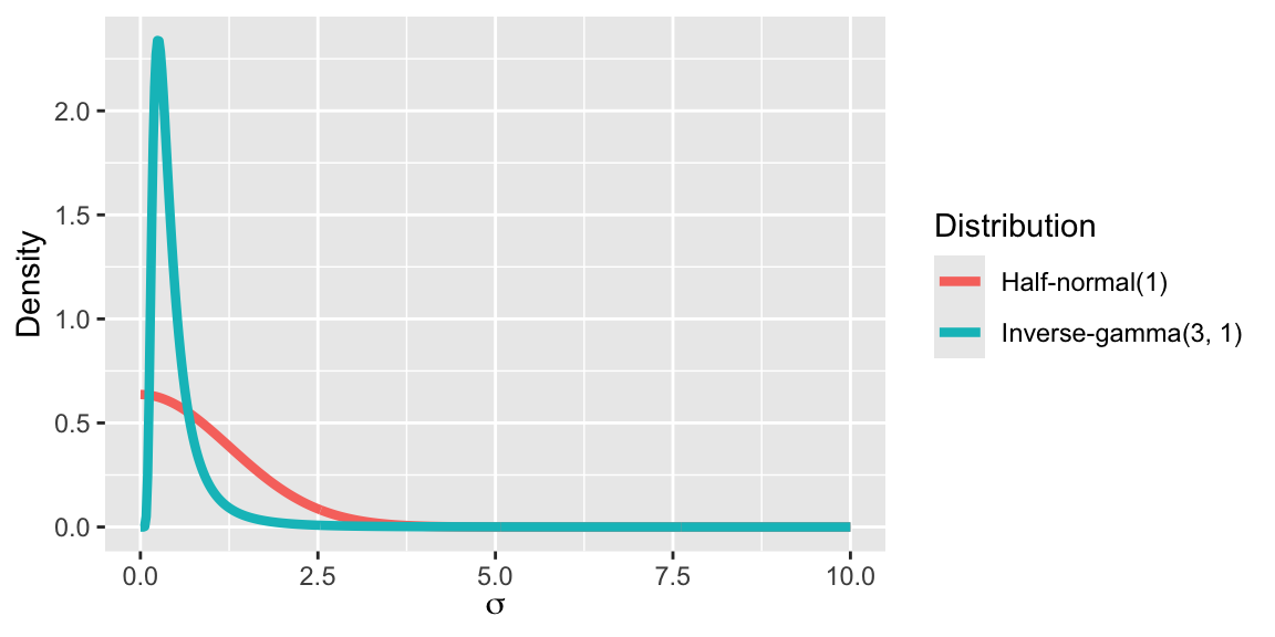
sigmais a half-normal distribution.
Quick aside
The half-normal is a useful prior for nonnegative parameters that should not be too large and may be very close to zero.
Similar distributions for scale parameters are half-t and half-Cauchy priors, these have heavier tales.
3. Check the model with simulated data:
Draw parameter values from priors.
Generate data based on those parameter values.
Check simulated data summaries and compare to observed data.
3. Check the model with simulated data:
// stored in workflow_prior_pred_check.stan
data {
int<lower = 1> n;
int<lower = 1> p;
real Y_bar;
matrix[n, p] X;
real<lower = 0> sigma_alpha;
real<lower = 0> sigma_beta;
real<lower = 0> sigma_sigma;
}
transformed data {
row_vector[p] X_bar;
for (i in 1:p) X_bar[i] = mean(X[, i]);
}
generated quantities {
// Sample from the priors
real alpha_star = normal_rng(0, sigma_alpha);
real alpha_plus = alpha_star + Y_bar;
real alpha = alpha_plus - X_bar * beta;
vector[p] beta;
for (i in 1:p) beta[i] = normal_rng(0, sigma_beta);
real sigma = fabs(normal_rng(0, sigma_sigma));
// Simulate data from the prior
vector[n] Y;
for (i in 1:n) {
Y[i] = normal_rng(alpha + X[i, ] * beta, sigma);
}
// Compute summaries from the prior
real Y_min = min(Y);
real Y_max = max(Y);
real Y_mean = mean(Y);
}3. Check the model with simulated data:
###Compile the Stan code
prior_check <- stan_model(file = "workflow_prior_pred_check.stan")
###Define the Stan data object
Y <- dat$weight
X <- matrix(dat$height)
stan_data <- list(
n = nrow(dat),
p = ncol(X),
Y_bar = mean(Y),
X = X,
sigma_alpha = 10,
sigma_beta = 10,
sigma_sigma = 10)
###Simulate data from the prior
prior_check1 <- sampling(prior_check, data = stan_data,
algorithm = "Fixed_param", chains = 1, iter = 1000)3. Check the model with simulated data:
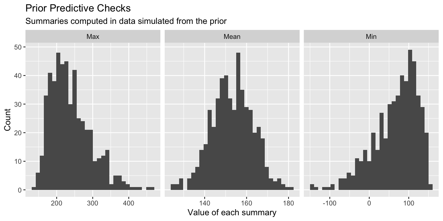
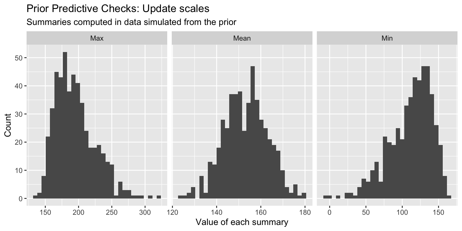
3. Check the model with simulated data:
###Compile the Stan code
prior_check <- stan_model(file = "workflow_prior_pred_check.stan")
###Define the Stan data object
Y <- dat$weight
X <- matrix(dat$height)
stan_data <- list(
n = nrow(dat),
p = ncol(X),
Y_bar = mean(Y),
X = X,
sigma_alpha = 10,
sigma_beta = 5,
sigma_sigma = 4)
###Simulate data from the prior
prior_check2 <- sampling(prior_check, data = stan_data,
algorithm = "Fixed_param", chains = 1, iter = 1000)3. Check the model with simulated data:
4. Fit the model to real data:
// saved in linear_regression_workflow.stan
data {
int<lower = 1> n; // number of observations
int<lower = 1> p; // number of covariates (excluding intercept)
vector[n] Y; // outcome vector
matrix[n, p] X; // covariate matrix
int<lower = 1> n_pred; // number of new observations to predict
matrix[n_pred, p] X_new; // covariate matrix for new observations
}
transformed data {
  vector[n] Y_centered;
  real Y_bar;
  matrix[n, p] X_centered;
  row_vector[p] X_bar;
  for (i in 1:p) {
    X_bar[i] = mean(X[, i]);
    X_centered[, i] = X[, i] - X_bar[i];
  }
  Y_bar = mean(Y);
  Y_centered = Y - Y_bar;
}
parameters {
real alpha_star;
vector[p] beta;
real<lower = 0> sigma;
}
model {
target += normal_lpdf(Y_centered | alpha_star + X_centered * beta, sigma); // likelihood
target += normal_lpdf(alpha_star | 0, 10);
target += normal_lpdf(beta | 0, 5);
sigma ~ normal(0, 4);
}
generated quantities {
vector[n] Y_pred;
vector[n] log_lik;
vector[n_pred] Y_new;
real alpha = Y_bar + alpha_star - X_bar * beta;
for (i in 1:n) {
Y_pred[i] = normal_rng(alpha + X[i, ] * beta, sigma);
log_lik[i] = normal_lpdf(Y_centered[i] | alpha_star + X_centered[i, ] * beta, sigma);
}
for (i in 1:n_pred) Y_new[i] = normal_rng(alpha + X_new[i, ] * beta, sigma);
}4. Fit the model to real data:
###Compile model
regression_model <- stan_model(file = "linear_regression_workflow.stan")

###Create data
Y <- dat$weight
X <- matrix(dat$height)
n_new <- 1000
X_new <- matrix(seq(min(dat$height), max(dat$height), length.out = n_new))
stan_data <- list(
  n = nrow(dat),
  p = ncol(X),
  Y = Y,
  X = X,
  n_new = n_new,
  X_new = X_new
)
4. Fit the model to real data:
Inference for Stan model: anon_model.
4 chains, each with iter=2000; warmup=1000; thin=1;
post-warmup draws per chain=1000, total post-warmup draws=4000.
mean se_mean sd 2.5% 50% 97.5% n_eff Rhat
alpha -230.32 0.25 16.71 -263.60 -230.48 -198.47 4349 1
beta[1] 5.68 0.00 0.25 5.20 5.68 6.17 4367 1
sigma 20.09 0.01 0.61 18.93 20.07 21.32 4148 1
Samples were drawn using NUTS(diag_e) at Mon Feb 3 13:39:30 2025.
For each parameter, n_eff is a crude measure of effective sample size,
and Rhat is the potential scale reduction factor on split chains (at
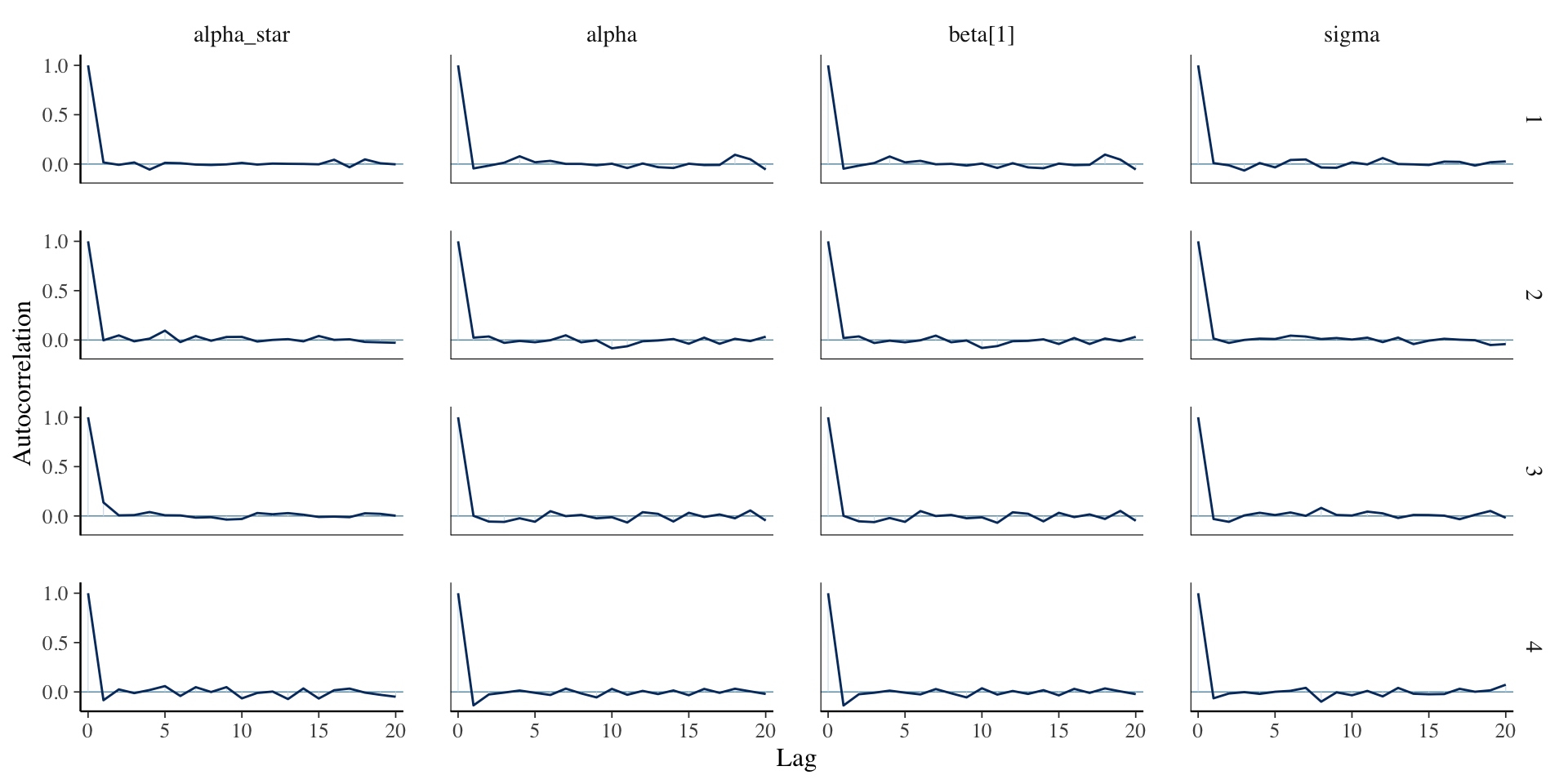
convergence, Rhat=1).5. Check diagnostics:
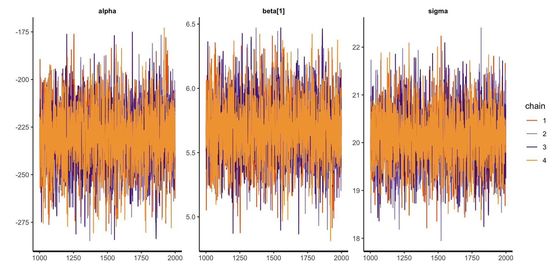
5. Check diagnostics:
6. Examine posterior fit:
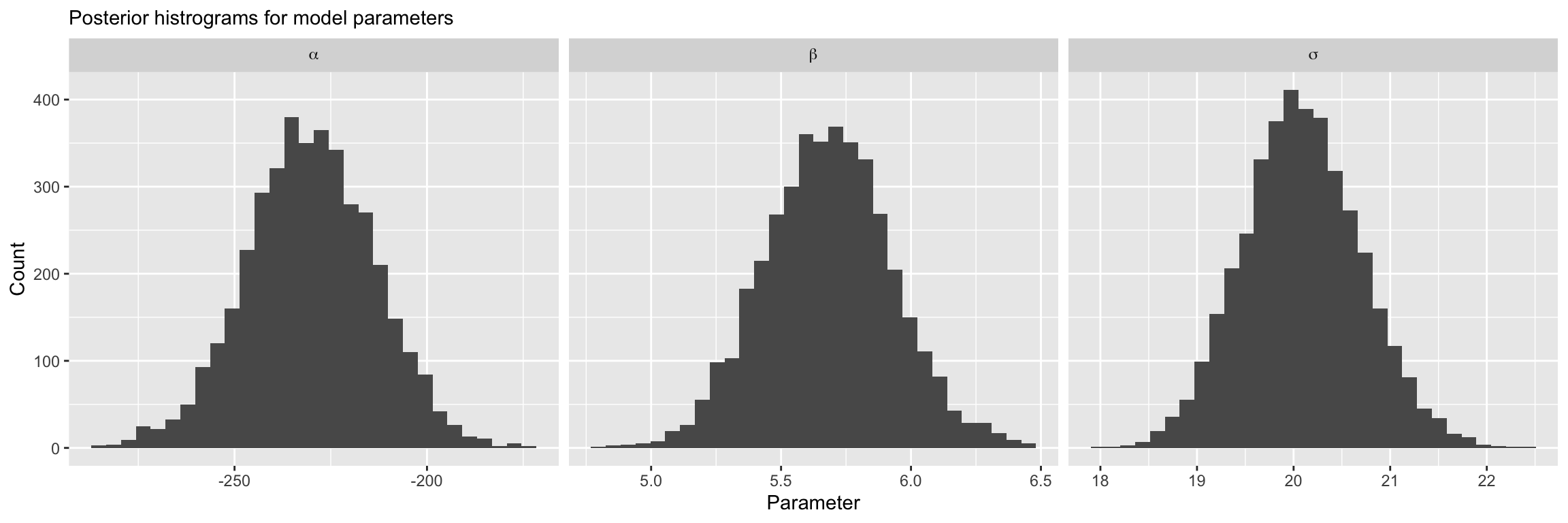
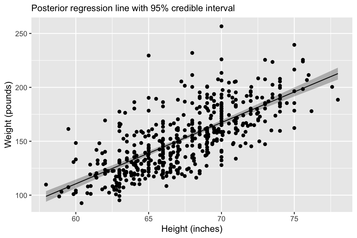
6. Examine posterior fit:

Regression line corresponds to posterior mean and 95% credible interval for \(\mu = \alpha + \mathbf{x}_i \boldsymbol{\beta}\).
6. Examine posterior fit:
7.Check predictions:
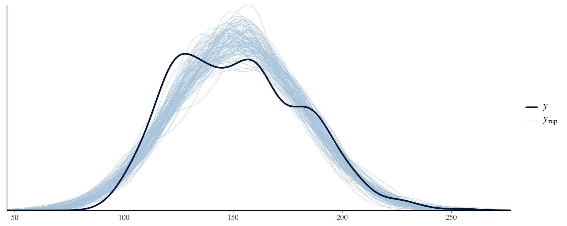
7. Check predictions:
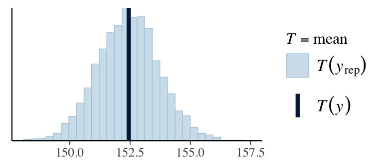
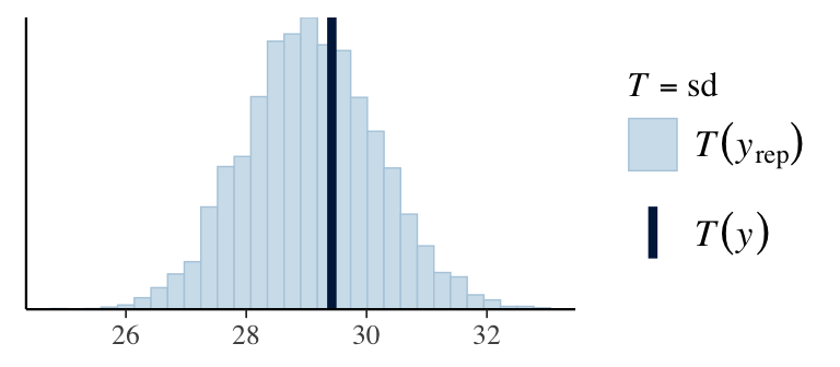
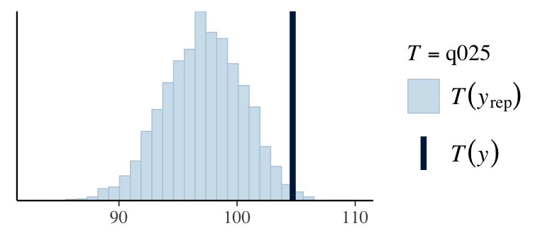
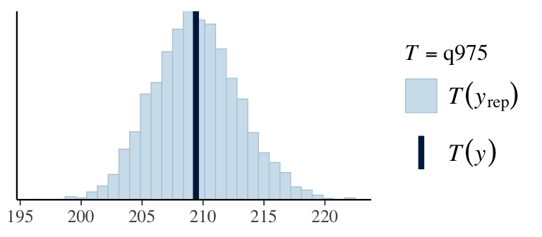
7. Check predictions:
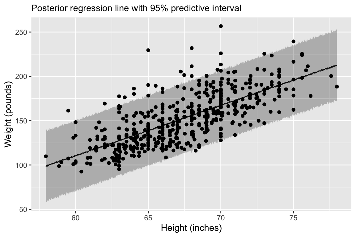
Regression line corresponds to posterior predictive distribution mean and 95% credible interval, \(f(Y_{i'} | Y_1,\ldots,Y_n)\).
shinystan
8. Compare models
- Suppose we would like to compare our original model with models that also includes sex and an interaction between sex and height.
\[\begin{aligned} \mathbb{E}[weight_i] &= \alpha + \beta_1 height_i\\ \mathbb{E}[weight_i] &= \alpha + \beta_1 height_i + \beta_2 sex_i\\ \mathbb{E}[weight_i] &= \alpha + \beta_1 height_i + \beta_2 sex_i + \beta_3 height_i sex_i \end{aligned}\]
8. Compare models
###Compute individual WAIC
library(loo)
log_lik_model1 <- loo::extract_log_lik(fit_model1, parameter_name = "log_lik", merge_chains = TRUE)
log_lik_model2 <- loo::extract_log_lik(fit_model2, parameter_name = "log_lik", merge_chains = TRUE)
log_lik_model3 <- loo::extract_log_lik(fit_model3, parameter_name = "log_lik", merge_chains = TRUE)
waic_model1 <- loo::waic(log_lik_model1)
waic_model2 <- loo::waic(log_lik_model2)
waic_model3 <- loo::waic(log_lik_model3)

###Make a comparison
comp_waic <- loo::loo_compare(list("height_only" = waic_model1, "height_sex" = waic_model2, "interaction" = waic_model3))
print(comp_waic, digits = 2, simplify = FALSE)
elpd_diff se_diff elpd_waic se_elpd_waic p_waic se_p_waic
interaction 0.00 0.00 -2225.62 24.22 5.08 0.96
height_sex -1.19 1.66 -2226.81 23.78 4.80 0.87
height_only -28.15 8.43 -2253.77 21.55 3.57 0.63
waic se_waic
interaction 4451.23 48.44
height_sex 4453.62 47.55
height_only 4507.53 43.108. Compare models
###Compute individual LOO-CV/LOO-IC
loo_model1 <- loo::loo(log_lik_model1)
loo_model2 <- loo::loo(log_lik_model2)
loo_model3 <- loo::loo(log_lik_model3)

###Make a comparison
comp_loo <- loo::loo_compare(list("height_only" = loo_model1, "height_sex" = loo_model2, "interaction" = loo_model3))
print(comp_loo, digits = 2, simplify = FALSE)
elpd_diff se_diff elpd_loo se_elpd_loo p_loo se_p_loo looic
interaction 0.00 0.00 -2225.63 24.23 5.10 0.96 4451.27
height_sex -1.18 1.66 -2226.81 23.78 4.80 0.87 4453.63
height_only -28.13 8.43 -2253.77 21.55 3.57 0.63 4507.54
se_looic
interaction 48.46
height_sex 47.56
height_only 43.10The plan moving forward
We have now learned all of the skills needed to implement a Bayesian workflow.
The remainder of the course will be focused on introducing new models for types of data that are common when working in the biomedical data setting.
Prepare for next class
Work on HW 02
Complete reading to prepare for next Thursday’s lecture
Thursday’s lecture: Nonlinear Regression