library(tidyverse)
library(rstan)
library(bayesplot)
library(knitr)
library(loo)
library(betareg)  # frequentist beta regression

# load other packages as neededLive-Coding
Beta regression for ED length of stay
Introduction
ImportantDue date
This live-coding exercise is to be completed in-class and turned in by Thursday, April 9 by 1:00 PM. To be considered on time, the following must be done by the due date:
- Final
.qmdand.pdffiles pushed to your GitHub repo - Final
.pdffile submitted on Gradescope
I will allow a 5-minute grace period, meaning assignments turned in by 1:05pm will be accepted, but nothing will be accepted after that time.
Live-Coding Session Details
- Date and Time: Thursday, April 9, 11:45 AM - 1:00 PM.
- Work Independently: You must work by yourself on this exercise. The teaching team will be available for questions.
- Resources Allowed:
- Lecture slides, homework, exercises, past exam, etc.
- Any material available online (research, textbooks, etc.).
- Restrictions:
- You cannot use AI to generate narrative or explanations during the session (you may use it for coding and technical queries).
The goal is to complete the task independently, applying everything you’ve learned so far in the course. Good luck!
Getting started
Go to the biostat725-sp26 organization on GitHub. Click on the repo with the prefix live-coding. It contains the starter documents you need to complete the live-coding exercise.
Clone the repo and start a new project in RStudio. See the AE 01 instructions for details on cloning a repo and starting a new project in R.
Packages
The following packages are used in this assignment:
Data
This live-coding exercise will use data from the MIMIC-IV-ED Demo, similar to the data from Exam 01 and the review live-coding. To obtain an analysis dataset, source the R script to obtain a dataset called live_coding.
source("live-coding-process-data.R")We will use the following variables from the dataset:
los: continuous, ED length of stay in hours.race: categorical with three levels,white,black, andother.arrival: categorical with two levels that reports mode of arrival to ED,ambulance, andwalk-in.sex: binary,femaleandmale.acuity_score: categorical with three levels that reports a patient’s level of emergency,stable,complex/high-risk, andmoderate-risk.o2sat: continuous, oxygen saturation in %.
Motivation
In Exam 01, we modeled ED length of stay using quantile regression and in the review for the live-coding we showed an example of using gamma regression (we also used a mixture model in the clustering lecture!). Today, we will consider yet another alternative modeling approach that uses beta regression. ED length of stay is given below, however we need to transform it to use beta regression.
live_coding |>
  ggplot(aes(x = los)) +
  geom_histogram() +
  labs(x = "ED Length of Stay (hours)",
       y = "Count")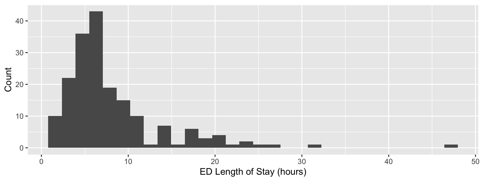
As a reminder, a beta distribution is appropriate for continuous random variables that are constrained to be between zero and one. In order to appropriately model ED length of stay as a beta random variable, we must convert the outcome variable into a proportion of hours stayed in the ED, which requires an upper bound (or denominator), which I specify as 2 days or 48 hours. Note that I already removed two patients with ED stays greater than 48 hours. The transformed outcome variable is given below.
live_coding |>
  ggplot(aes(x = los / 48)) +
  geom_histogram() +
  labs(x = "Normalized ED length of stay (ED LOS divided by 48 hours)",
       y = "Count")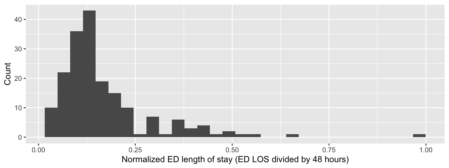
This outcome variable makes it a nice candidate for beta regression because it is continuous and constrained between zero and one. In this live-coding exercise we will implement beta regression for ED length of stay using a logit link function.
Beta regression
Definition of Beta Random Variable
A random variable \(Y\) with shape \(\alpha > 0\) and shape \(\theta > 0\) can be written as \(Y \sim \text{Beta}(\alpha, \theta)\) with density \(f_Y(y | \alpha, \theta) = B(\alpha,\theta)^{-1}y^{\alpha-1}(1-y)^{\theta-1}\), where \(B(\alpha,\theta) = [\Gamma(\alpha)\Gamma(\theta)]/\Gamma(\alpha + \theta)\) is the beta function. The mean and variance are given by: \(\mathbb{E}[Y] = \alpha/(\alpha + \theta) = \mu\) and \(\mathbb{V}(Y) = (\alpha\theta) / [(\alpha + \theta)^2(\alpha + \theta + 1)]\). One way to perform regression for a beta distributed random variable is to make a change-of-variables so that the density is parameterized in terms of the mean \(\mu = \alpha/(\alpha + \theta)\) and a precision parameter \(\phi = \alpha + \theta\), such that \(\alpha=\mu\phi\) and \(\theta=(1-\mu)\phi\). Under this specification, \(\mathbb{E}[Y] = \mu\) and \(\mathbb{V}(Y) = [\mu(1-\mu)] / (\phi + 1)\).
To perform beta regression, predictors are related to the mean using a logit link function, \(\text{logit} (\mu_i) = \log\left[\mu_i/(1-\mu_i)\right] = \alpha + \mathbf{x}_i \boldsymbol{\beta}\). Thus, the full model can be written as,
\[\begin{align*} Y_i &\stackrel{ind}{\sim} \text{Beta}(\mu_i, \phi),\quad i = 1,\ldots,n\\ \text{logit}(\mu_i) &= \alpha + \mathbf{x}_i \boldsymbol{\beta}\\ \boldsymbol{\Omega} &\sim f(\boldsymbol{\Omega}),\\ \end{align*}\]
where \(\boldsymbol{\Omega} = (\alpha, \boldsymbol{\beta}, \phi)\).
Interpreting Coefficients
In this beta regression, we model the mean of the outcome (the normalized ED length of stay) using a logit link: \(\text{logit}(\mu_i) = \alpha + \mathbf{x}_i \boldsymbol{\beta}\). This means that each coefficient \(\beta_j\) represents a change in the log-odds of the mean proportion for a one-unit increase in predictor \(x_j\), holding all other variables constant. When we exponentiate the coefficients, \(\gamma_j = \exp\{\beta_j\}\), we obtain an odds ratio.
Importantly, we’re calling these “odds ratios”, but they are not odds of an event happening like in logistic regression. In logistic regression, odds come from a probability of a binary outcome (e.g., success vs. failure). Here, our outcome is continuous between zero and one, and we are modeling the average level of that outcome. So when we exponentiate the coefficients, we are getting multiplicative changes in the odds of the mean proportion, not the odds of an event. The math is the same as in logistic regression, but the interpretation is different: these describe how predictors shift the average proportion, not the probability of an event.
Exercises
We are interested in fitting a beta regression to the the normalized ED length of stay, defined as \(Y_i\) for \(i = 1,\ldots,n\). We would like to fit the following model,
\[\begin{align*} Y_i &\stackrel{ind}{\sim} \text{Beta}(\mu_i, \phi)\\ \text{logit}(\mu_i) &= \alpha + \mathbf{x}_i\boldsymbol{\beta}\\ &= \alpha + \beta_1 black_i + \beta_2 other_i + \beta_3 arrival\_walkin_i\\ &\quad+ \beta_4 male_i + \beta_5 acuity\_score\_moderate_i\\ &\quad+ \beta_6 acuity\_score\_complex_i + \beta_7 o2sat_i. \end{align*}\]
When you fit the model, make sure to center the predictors, such that \(\text{logit}(\mu_i) = \alpha^* + \mathbf{x}_i^* \boldsymbol{\beta}\), where \(\mathbf{x}_i^* = \mathbf{x}_i - \bar{\mathbf{x}}\) and \(\bar{\mathbf{x}} = \frac{1}{n}\sum_{i=1}^n \mathbf{x}_i\). Use the following priors \(\alpha^* \sim N(0,5^2)\), \(\beta_j \stackrel{iid}{\sim} N(0,5^2)\), \(j = 1,\ldots,p\) and \(\phi \sim \mathcal C^+(5^2)\), which is a half-Cauchy with scale 5.
ImportantStan code
In your repo you will find a Stan script called live-coding.stan. This will act as your starter script for performing beta regression. Throughout Exercises 1-4 you will be prompted to add lines of code to the Stan script and in Exercises 5-9 you will use your completed Stan code.
Exercise 1
To perform beta regression in Stan, we will create a function in your Stan code called beta_regression_lpdf that encodes the log-likelihood function using the parameterization \(Y_i \stackrel{ind}{\sim} \text{Beta}(\mu_i,\phi)\). In order to do this use the pre-defined beta random variable that is built into Stan. To answer this question, print the function you created using a {stan output.var = "likelihood", eval = FALSE} code chunk. While not required, the function beta_regression_lpdf should be vectorized to be consistent with its use in the model code chunk. You should only have to modify line 4 of the Stan code.
Exercise 2
Building on Exercise 1, we would like to create a function called beta_regression_rng that will permit sampling from the posterior predictive distribution. Be sure to use the built in beta_rng function. The function beta_regression_rng should not be vectorized. To answer this question, print the function you created using a {stan output.var = "rng", eval = FALSE} code chunk. You should only have to modify line 8 of the Stan code.
Exercise 3
We now need to define the mean process for the beta regression model. Recall that in this model, the outcome mean is linked to the predictors through a logit link, so that the mean normalized ED length of stay depends on the linear predictor formed from the centered design matrix and regression coefficients. To answer this question, fill in the line that defines mu in the transformed parameters block of the Stan code. Your answer should use the built in inv_logit function. To answer this question, print the line you created using a {stan output.var = "mu", eval = FALSE} code chunk. You should only have to modify line 33 of the Stan code.
Exercise 4
We now want to generate a draw from the posterior predictive distribution for a new observation with covariate values given by X_new. Recall that the posterior predictive distribution is obtained by first computing the mean outcome for the new set of covariates and then drawing a new value from the beta regression model using that mean (\(\mu_i\)) and the precision parameter \(\phi\). To answer this question, fill in the line that defines Y_new in the generated quantities block of the Stan code. Your answer should use the function beta_regression_rng that you created in Exercise 2. To answer this question, print the line you created using a {stan output.var = "Y_new", eval = FALSE} code chunk. You should only have to modify line 50 of the Stan code.
Exercise 5
Using the code from the previous exercises, fit the beta regression model specified above. Make a statement about MCMC convergence for \(\alpha\), \(\boldsymbol{\beta}\), and \(\phi\) based on MC standard error, effective sample size, \(\hat{R}\), traceplots, and autocorrelation.
Exercise 6
Present posterior means and 95% intervals for \(\alpha\), \(\boldsymbol{\beta}\), and \(\phi\). One way to verify that the model has converged is to compare the results with an analogous frequentist model as a sanity check. The beta regression with logit link function can be computed as: summary(betareg(I(los / 48) ~ race + arrival + sex + acuity_score + o2sat, data = live_coding)). Are the Bayesian and frequentist results consistent?
Exercise 7
Perform a posterior predictive check to assess model fit and describe how well the model fits the data.
Exercise 8
Consider a patient who is black, arrived by ambulance, is male, has a complex/high-risk condition, and has an oxygen saturation of 98. Define the corresponding covariate vector X_new, obtain posterior predictive draws of Y_new, and report the posterior predictive mean and a 95% interval. Finally, also report the mean and 95% interval on the original scale (hours).
Exercise 9
Present posterior summaries for \(\gamma_j\) for \(j=1,\ldots,p\). Provide an interpretation for \(\gamma_4\) (male) within the context of the scientific problem.
Submission
You will submit the PDF documents for the live-coding to Gradescope as part of your final submission.
Warning
Before you wrap up the exercise, make sure all documents are updated on your GitHub repo.
Remember – you must turn in a PDF file to the Gradescope page before the submission deadline for full credit.
To submit your assignment:
Access Gradescope through the menu on the BIOSTAT 725 Canvas site.
Click on the assignment, and you’ll be prompted to submit it.
Mark the pages associated with each exercise. All of the pages of your live-coding should be associated with at least one question (i.e., should be “checked”).
Grading
| Component | Points |
|---|---|
| Ex 1 | 8 |
| Ex 2 | 7 |
| Ex 3 | 5 |
| Ex 4 | 5 |
| Ex 5 | 5 |
| Ex 6 | 5 |
| Ex 7 | 5 |
| Ex 8 | 5 |
| Ex 9 | 5 |